Stronger net selection on males across animals
Supplementary material reporting R code
Lennart Winkler1, Maria Moiron2, Edward H. Morrow3 and Tim Janicke1,2
1Applied Zoology, Technical University Dresden
2Centre d’Écologie Fonctionnelle et Évolutive, UMR 5175, CNRS, Université de Montpellier 3Department for Environmental and Life Sciences, Karlstad University
Last updated: 2021-09-27
Checks: 7 0
Knit directory: Net_Selection_eLife_code/
This reproducible R Markdown analysis was created with workflowr (version 1.6.2). The Checks tab describes the reproducibility checks that were applied when the results were created. The Past versions tab lists the development history.
Great! Since the R Markdown file has been committed to the Git repository, you know the exact version of the code that produced these results.
Great job! The global environment was empty. Objects defined in the global environment can affect the analysis in your R Markdown file in unknown ways. For reproduciblity it’s best to always run the code in an empty environment.
The command set.seed(20210613) was run prior to running the code in the R Markdown file. Setting a seed ensures that any results that rely on randomness, e.g. subsampling or permutations, are reproducible.
Great job! Recording the operating system, R version, and package versions is critical for reproducibility.
Nice! There were no cached chunks for this analysis, so you can be confident that you successfully produced the results during this run.
Great job! Using relative paths to the files within your workflowr project makes it easier to run your code on other machines.
Great! You are using Git for version control. Tracking code development and connecting the code version to the results is critical for reproducibility.
The results in this page were generated with repository version a6602c7. See the Past versions tab to see a history of the changes made to the R Markdown and HTML files.
Note that you need to be careful to ensure that all relevant files for the analysis have been committed to Git prior to generating the results (you can use wflow_publish or wflow_git_commit). workflowr only checks the R Markdown file, but you know if there are other scripts or data files that it depends on. Below is the status of the Git repository when the results were generated:
Ignored files:
    Ignored:    .Rhistory
    Ignored:    data/.Rhistory

Untracked files:
    Untracked:  data/Winkler_et_al_2021_eLife_DataTable.txt
    Untracked:  data/Winkler_et_al_2021_eLife_Phylogeny.txt
    Untracked:  data/Winkler_et_al_2021_eLife_Phylogeny_PIC.txt
Note that any generated files, e.g. HTML, png, CSS, etc., are not included in this status report because it is ok for generated content to have uncommitted changes.
These are the previous versions of the repository in which changes were made to the R Markdown (analysis/index.Rmd) and HTML (docs/index.html) files. If you’ve configured a remote Git repository (see ?wflow_git_remote), click on the hyperlinks in the table below to view the files as they were in that past version.
| File | Version | Author | Date | Message |
|---|---|---|---|---|
| Rmd | a6602c7 | LennartWinkler | 2021-09-27 | wflow_publish(republish = TRUE, all = T) |
| html | 3b9b079 | LennartWinkler | 2021-09-22 | Build site. |
| html | dcdf568 | LennartWinkler | 2021-09-22 | Build site. |
| Rmd | 1d415ea | LennartWinkler | 2021-09-22 | wflow_publish(republish = TRUE, all = T) |
| html | 1d415ea | LennartWinkler | 2021-09-22 | wflow_publish(republish = TRUE, all = T) |
| Rmd | f1eb5c9 | LennartWinkler | 2021-09-22 | wflow_publish(all = T) |
| html | f1eb5c9 | LennartWinkler | 2021-09-22 | wflow_publish(all = T) |
| html | 0f87db4 | LennartWinkler | 2021-06-23 | Build site. |
| Rmd | b46a782 | LennartWinkler | 2021-06-23 | wflow_publish(all = T) |
| html | b46a782 | LennartWinkler | 2021-06-23 | wflow_publish(all = T) |
| html | 79ae987 | LennartWinkler | 2021-06-23 | Build site. |
| Rmd | f7593bd | LennartWinkler | 2021-06-23 | wflow_publish(all = T) |
| html | f7593bd | LennartWinkler | 2021-06-23 | wflow_publish(all = T) |
| html | 98c553d | LennartWinkler | 2021-06-23 | Build site. |
| Rmd | 926ceb8 | LennartWinkler | 2021-06-23 | wflow_publish(all = T) |
| html | 926ceb8 | LennartWinkler | 2021-06-23 | wflow_publish(all = T) |
| html | 3bccaab | LennartWinkler | 2021-06-23 | Build site. |
| Rmd | 7ffcf00 | LennartWinkler | 2021-06-23 | wflow_publish(all = T) |
| html | 7ffcf00 | LennartWinkler | 2021-06-23 | wflow_publish(all = T) |
| html | 63df934 | LennartWinkler | 2021-06-23 | Build site. |
| Rmd | 36c6fdc | LennartWinkler | 2021-06-23 | wflow_publish(all = T) |
| html | 36c6fdc | LennartWinkler | 2021-06-23 | wflow_publish(all = T) |
| html | b3577de | LennartWinkler | 2021-06-23 | Build site. |
| Rmd | 85c0b6e | LennartWinkler | 2021-06-23 | wflow_publish(all = T) |
| html | 85c0b6e | LennartWinkler | 2021-06-23 | wflow_publish(all = T) |
| html | 4ed93cf | LennartWinkler | 2021-06-23 | Build site. |
| Rmd | 058af7b | LennartWinkler | 2021-06-23 | wflow_publish(all = T) |
| html | 058af7b | LennartWinkler | 2021-06-23 | wflow_publish(all = T) |
| html | 223df21 | LennartWinkler | 2021-06-23 | Build site. |
| Rmd | f63b665 | LennartWinkler | 2021-06-23 | wflow_publish(all = T) |
| html | f63b665 | LennartWinkler | 2021-06-23 | wflow_publish(all = T) |
| html | 3139eb4 | LennartWinkler | 2021-06-14 | Build site. |
| Rmd | 9290105 | LennartWinkler | 2021-06-14 | wflow_publish(all = TRUE) |
| html | 9290105 | LennartWinkler | 2021-06-14 | wflow_publish(all = TRUE) |
| html | 01525f8 | LennartWinkler | 2021-06-13 | Build site. |
| Rmd | 161eee9 | LennartWinkler | 2021-06-13 | wflow_publish(“C:/Users/lenna/Desktop/Documents/PhD/2020_META SexSpecGenVar/eLife/Net_Selection_eLife_code/analysis/index.Rmd”) |
| html | 6f60c27 | LennartWinkler | 2021-06-13 | Build site. |
| Rmd | 555a290 | LennartWinkler | 2021-06-13 | wflow_publish(“C:/Users/lenna/Documents/Net_Selection_eLife_code/analysis/index.Rmd”) |
| html | 9220292 | LennartWinkler | 2021-06-13 | Build site. |
| Rmd | 15f14fe | LennartWinkler | 2021-06-13 | wflow_publish(“C:/Users/lenna/Documents/Net_Selection_eLife_code/analysis/index.Rmd”) |
| html | db2f16f | LennartWinkler | 2021-06-13 | Build site. |
| Rmd | 00738af | LennartWinkler | 2021-06-13 | wflow_publish(“C:/Users/lenna/Documents/Net_Selection_eLife_code/analysis/index.Rmd”) |
| html | 7d5ef2c | LennartWinkler | 2021-06-13 | Build site. |
| Rmd | 320011b | LennartWinkler | 2021-06-13 | Start workflowr project. |
Supplementary material reporting R code for the manuscript ‘Stronger net selection on males across animals’.
Load and prepare data
Before we started the analyses, we loaded all necessary packages and data. All data have been published at https://zenodo.org/record/5529490#.YVFnzlObE0N.
#load packages
rm(list = ls())
library(ape)
library(MCMCglmm)
library(caper) #for phylogenetic independent contrasts (PICs)
library(tidyr)
library(matrixcalc)
library(lattice)
library(ggplot2)
library(reshape2)

#load data
setwd(".")
Data <- read.delim("./data/Winkler_et_al_2021_eLife_DataTable.txt")
theTree <- read.tree("./data/Winkler_et_al_2021_eLife_Phylogeny.txt") #phylogenetic tree
#Load phylogenetic tree for PIC analyses
PIC_Tree <- read.tree("./data/Winkler_et_al_2021_eLife_Phylogeny_PIC.txt")

## Reorganising and subsetting dataset ####

stacked_gen_Data <- gather(Data, key = "Sex",value = "genCV", genCV_male, genCV_female)
stacked_phen_Data <- gather(Data, key = "Sex",value = "phenCV", phenCV_male, phenCV_female)

RS_gen_metaData<-subset(stacked_gen_Data, FitnessCat == "RS")
LS_gen_metaData<-subset(stacked_gen_Data, FitnessCat == "LS")

RS_phen_metaData<-subset(stacked_phen_Data, FitnessCat == "RS")
LS_phen_metaData<-subset(stacked_phen_Data, FitnessCat == "LS")

RS_Data<-subset(Data, FitnessCat == "RS")
LS_Data<-subset(Data, FitnessCat == "LS")
Phenotypic gambit
Statistical analyses were carried out in two steps. First, we examined the key assumption of the ‘phenotypic gambit’ by testing whether estimates of phenotypic variance predict the estimated genetic variance. For this we ran linear regressions with CVP defined as predictor variable and CVG defined as response variable. This was done separately for both sexes and the two fitness components. The analyses on the phenotypic gambit were motivated from a methodological perspective and we did not expect that inter-specific variation in the difference between CVP and CVG can be explained by a shared phylogenetic history. However, for completeness, we also ran linear regressions on phylogenetic independent contrasts (PICs) computed using the crunch function of the caper R-package (version 1.0.1) in R (Orme et al. 2018) to test whether our findings were robust when accounting for potential phylogenetic non-independence.
First, we computed linear regressions between genetic and phenotypic variances, not controlling for the phylogeny. We started with the linear regression in reproductive success for males.
### Linear regressions (not controlling for phylogeny) ####

LM_Gambit_RS_males   <- lm(genCV_male   ~ phenCV_male,   data = RS_Data) #Reproductive success in males
summary(LM_Gambit_RS_males) #Reproductive success in males
Call:
lm(formula = genCV_male ~ phenCV_male, data = RS_Data)

Residuals:
     Min       1Q   Median       3Q      Max
-0.39325 -0.13953 -0.08111  0.11677  0.62956

Coefficients:
            Estimate Std. Error t value Pr(>|t|)
(Intercept)  0.24747    0.06078   4.071 0.000139 ***
phenCV_male  0.08514    0.05981   1.423 0.159792
---
Signif. codes:  0 '***' 0.001 '**' 0.01 '*' 0.05 '.' 0.1 ' ' 1

Residual standard error: 0.2214 on 60 degrees of freedom
Multiple R-squared:  0.03267,   Adjusted R-squared:  0.01654
F-statistic: 2.026 on 1 and 60 DF,  p-value: 0.1598
Then we continued with the linear regression in reproductive success for females.
LM_Gambit_RS_females <- lm(genCV_female ~ phenCV_female, data = RS_Data) #Reproductive success in females
summary(LM_Gambit_RS_females) #Reproductive success in females
Call:
lm(formula = genCV_female ~ phenCV_female, data = RS_Data)

Residuals:
     Min       1Q   Median       3Q      Max
-0.24799 -0.10236 -0.02864  0.07889  0.54843

Coefficients:
              Estimate Std. Error t value Pr(>|t|)
(Intercept)    0.21221    0.04865   4.362 5.14e-05 ***
phenCV_female  0.03832    0.06480   0.591    0.556
---
Signif. codes:  0 '***' 0.001 '**' 0.01 '*' 0.05 '.' 0.1 ' ' 1

Residual standard error: 0.1755 on 60 degrees of freedom
Multiple R-squared:  0.005795,  Adjusted R-squared:  -0.01077
F-statistic: 0.3497 on 1 and 60 DF,  p-value: 0.5565
Next, the linear regression in lifespan for males.
LM_Gambit_LS_males   <- lm(genCV_male   ~ phenCV_male,   data = LS_Data) #Lifespan in males
summary(LM_Gambit_LS_males) #Lifespan in males
Call:
lm(formula = genCV_male ~ phenCV_male, data = LS_Data)

Residuals:
      Min        1Q    Median        3Q       Max
-0.200220 -0.059558  0.006778  0.048454  0.260075

Coefficients:
            Estimate Std. Error t value Pr(>|t|)
(Intercept)  0.04934    0.02969   1.662 0.104960
phenCV_male  0.26577    0.06794   3.912 0.000378 ***
---
Signif. codes:  0 '***' 0.001 '**' 0.01 '*' 0.05 '.' 0.1 ' ' 1

Residual standard error: 0.09687 on 37 degrees of freedom
Multiple R-squared:  0.2926,    Adjusted R-squared:  0.2734
F-statistic:  15.3 on 1 and 37 DF,  p-value: 0.0003778
Finally, the linear regression in lifespan for females.
LM_Gambit_LS_females <- lm(genCV_female ~ phenCV_female, data = LS_Data) #Lifespan in females
summary(LM_Gambit_LS_females) #Lifespan in females
Call:
lm(formula = genCV_female ~ phenCV_female, data = LS_Data)

Residuals:
     Min       1Q   Median       3Q      Max
-0.16792 -0.05745  0.01441  0.04686  0.15623

Coefficients:
              Estimate Std. Error t value Pr(>|t|)
(Intercept)    0.05455    0.02248   2.426 0.020245 *
phenCV_female  0.20435    0.05083   4.020 0.000275 ***
---
Signif. codes:  0 '***' 0.001 '**' 0.01 '*' 0.05 '.' 0.1 ' ' 1

Residual standard error: 0.0733 on 37 degrees of freedom
Multiple R-squared:  0.304, Adjusted R-squared:  0.2852
F-statistic: 16.16 on 1 and 37 DF,  p-value: 0.0002749
Next, we expanded the previous analyses on the phenotypic gambit, by considering the phylogeny using phylogenetic independent contrasts (PICs).
# Phylogenetic linear regressions using the caper package ####

#Build phylogenetic tree for reproductive success
RS_Data$Species_PIC <- factor(RS_Data$Species_PIC)
RS_Species_Data_PIC <- unique(RS_Data$Species_PIC)
RS_PIC_Tree<-drop.tip(PIC_Tree, PIC_Tree$tip.label[-na.omit(match(RS_Species_Data_PIC, PIC_Tree$tip.label))])
plot(RS_PIC_Tree)
#Build phylogenetic tree for lifespan
LS_Data$Species_PIC <- factor(LS_Data$Species_PIC)
LS_Species_Data_PIC <- unique(LS_Data$Species_PIC)
LS_PIC_Tree<-drop.tip(PIC_Tree, PIC_Tree$tip.label[-na.omit(match(LS_Species_Data_PIC, PIC_Tree$tip.label))])
plot(LS_PIC_Tree)#Combine phylogeny and data
PGLS_RS_Data <-comparative.data(phy = RS_PIC_Tree, data = RS_Data, names.col = Species_PIC, vcv = TRUE, na.omit = FALSE, warn.dropped = TRUE)
PGLS_LS_Data <-comparative.data(phy = LS_PIC_Tree, data = LS_Data, names.col = Species_PIC, vcv = TRUE, na.omit = FALSE, warn.dropped = TRUE)
#Run PIC using caper package
PIC_Crunch_mRS <- crunch(genCV_male ~ phenCV_male, data=PGLS_RS_Data, equal.branch.length=FALSE)
PIC_Crunch_fRS <- crunch(genCV_female ~ phenCV_female, data=PGLS_RS_Data, equal.branch.length=FALSE)
PIC_Crunch_mLS <- crunch(genCV_male ~ phenCV_male, data=PGLS_LS_Data, equal.branch.length=FALSE)
PIC_Crunch_fLS <- crunch(genCV_female ~ phenCV_female, data=PGLS_LS_Data, equal.branch.length=FALSE)
PIC_Crunch_mRS #PIC male reproductive success
PIC_Crunch_fRS #PIC female reproductive success
PIC_Crunch_mLS #PIC male lifespan
PIC_Crunch_fLS #PIC female lifespanThe results for phylogenetic independent contrast (PIC) for male reproductive success:
Phylogenetic Independent Contrasts analysis using:crunch.
Response values are species rich contrasts using:

Phylogeny:  (62 tips)
Data:  (62 rows)
Number of valid contrasts: 61

Call:
lm(genCV_male ~ phenCV_male - 1, data = contrData)

Residuals:
    Min      1Q  Median      3Q     Max
-5.3797 -0.0128  0.0685  1.1351  7.6022

Coefficients:
            Estimate Std. Error t value Pr(>|t|)
phenCV_male  0.11328    0.05145   2.202   0.0315 *
---
Signif. codes:  0 '***' 0.001 '**' 0.01 '*' 0.05 '.' 0.1 ' ' 1

Residual standard error: 2.071 on 60 degrees of freedom
Multiple R-squared:  0.07475,   Adjusted R-squared:  0.05933
F-statistic: 4.847 on 1 and 60 DF,  p-value: 0.03155
The results for phylogenetic independent contrast (PIC) for female reproductive success:
Phylogenetic Independent Contrasts analysis using:crunch.
Response values are species rich contrasts using:

Phylogeny:  (62 tips)
Data:  (62 rows)
Number of valid contrasts: 61

Call:
lm(genCV_female ~ phenCV_female - 1, data = contrData)

Residuals:
    Min      1Q  Median      3Q     Max
-4.4166 -0.1539  0.0011  0.5176  3.7100

Coefficients:
              Estimate Std. Error t value Pr(>|t|)
phenCV_female  0.19087    0.06503   2.935  0.00472 **
---
Signif. codes:  0 '***' 0.001 '**' 0.01 '*' 0.05 '.' 0.1 ' ' 1

Residual standard error: 1.498 on 60 degrees of freedom
Multiple R-squared:  0.1256,    Adjusted R-squared:  0.111
F-statistic: 8.615 on 1 and 60 DF,  p-value: 0.00472
The results for phylogenetic independent contrast (PIC) for male lifespan:
Phylogenetic Independent Contrasts analysis using:crunch.
Response values are species rich contrasts using:

Phylogeny:  (39 tips)
Data:  (39 rows)
Number of valid contrasts: 38

Call:
lm(genCV_male ~ phenCV_male - 1, data = contrData)

Residuals:
     Min       1Q   Median       3Q      Max
-1.23024 -0.03652 -0.00295  0.24827  1.80770

Coefficients:
            Estimate Std. Error t value Pr(>|t|)
phenCV_male  0.55262    0.04826   11.45 1.01e-13 ***
---
Signif. codes:  0 '***' 0.001 '**' 0.01 '*' 0.05 '.' 0.1 ' ' 1

Residual standard error: 0.5219 on 37 degrees of freedom
Multiple R-squared:  0.7799,    Adjusted R-squared:  0.774
F-statistic: 131.1 on 1 and 37 DF,  p-value: 1.008e-13
The results for phylogenetic independent contrast (PIC) for female lifespan:
Phylogenetic Independent Contrasts analysis using:crunch.
Response values are species rich contrasts using:

Phylogeny:  (39 tips)
Data:  (39 rows)
Number of valid contrasts: 38

Call:
lm(genCV_female ~ phenCV_female - 1, data = contrData)

Residuals:
     Min       1Q   Median       3Q      Max
-1.19148 -0.01920 -0.00039  0.31029  1.23392

Coefficients:
              Estimate Std. Error t value Pr(>|t|)
phenCV_female  0.34523    0.03616   9.547  1.6e-11 ***
---
Signif. codes:  0 '***' 0.001 '**' 0.01 '*' 0.05 '.' 0.1 ' ' 1

Residual standard error: 0.4447 on 37 degrees of freedom
Multiple R-squared:  0.7112,    Adjusted R-squared:  0.7034
F-statistic: 91.14 on 1 and 37 DF,  p-value: 1.6e-11
Stronger net selection on males (PGLMMs)
In this second part of the analysis, we tested the hypothesis that net selection is stronger on males by testing for a male bias in CVP and CVG. Specifically, we ran Phylogenetic General Linear Mixed-Effects Models (PGLMMs) with CVP or CVG as the response variable, and sex as a fixed effect. To account for the paired data structure, we added an observation identifier as a random effect. Moreover, all models included a study identifier and the phylogeny (transformed into a correlation matrix) as random effects to account for statistical non-independence arising from shared study design or phylogenetic history, respectively. Note that the latter also accounts for the non-independence of estimates obtained from the same species as some studies estimated genetic variances from distinct field populations (Fox et al. 2004) or different experimental treatments under laboratory conditions such as food stress (Holman & Jacomb 2017) and temperature stress (Berger et al. 2014). In an additional series of PGLMMs we tested whether our proxy of sexual selection explained inter-specific variation in the sex-differences of CVP or CVG by adding mating system and its interaction with sex as fixed effects to the models. These analyses were run on both the complete dataset and on a subset including only vertebrates. The latter set of analyses were done to acknowledge the fact that all sampled invertebrate species were classified as polygamous and the three independent evolutionary events in our phylogeny marking transitions between mating systems occurred in vertebrates (including 6 polygamous species, 6 monogamous species). Finally, given that primary studies varied in several methodological aspects (see section ‘Literature Search and Characterization of Primary Studies’) and whenever the level of replication allowed statistical analysis, we tested whether the different approaches predicted estimates of CVP and CVG and affected their sex-difference. Specifically, we ran three PGLMMs to test separately for effects of the study type, the estimate of genetic variance VG, and the type of reproductive success metric (see above). We carried out PGLMMs with the MCMCglmm R-package (version 2.2.9) (Hadfield 2010), using uninformative priors (V = 1, nu = 0.01) and an effective sample size of 20000 (number of iterations = 11000000, burn-in = 1000000, thinning interval = 500). We computed the proportion of variance explained by fixed factors (‘marginal R2’) (Nakagawa & Schielzeth 2013). In addition, we quantified the phylogenetic signal as the phylogenetic heritability H2 (i.e., proportional variance in CVP or CVG explained by the phylogeny) (de Villemereuil & Nakagawa 2014). In a previous study testing for sex-specific phenotypic variances in reproductive success (Janicke et al. 2016), we ran formal meta-analyses using lnCVR as the tested effect size (Nakagawa et al. 2015). This is potentially a more powerful approach for comparing phenotypic variances but rendered unsuitable when comparing genetic variances. This is because the computation of the sampling variance of lnCVR is a function of the sample size of the sampled population and the point estimate of lnCVR (Nakagawa et al. 2015). However, genetic variances are estimates from statistical models and notorious for being estimated with low precision (i.e., have large confidence intervals). Therefore, using a meta-analytic approach for genetic variances using lnCVR as an effect size leads to overconfident estimation of the global effect size and is therefore likely to result in type-II-errors. However, to allow comparison with the previous meta-analysis, we report the outcome of phylogenetic meta-analyses on phenotypic variances using lnCVR in the Supplementary Material (Table S3), which largely reflects the results on the point estimates of CVP from PGLMMs.
Run MCMC models
We then ran MCMC models to test for differences in the phenotypic and genetic variances in males and females for the fitness categories reproductive success and lifespan.
First, we pruned the phylogenetic tree to the data subset.
## PRUNE PHYLOGENETIC TREE TO DATA SUBSET
RS_gen_metaData$animal <- factor(RS_gen_metaData$animal)
is.factor(RS_gen_metaData$animal)
RS_Species_Data <- unique(RS_gen_metaData$animal)
summary(RS_Species_Data)
RS_theTree<-drop.tip(theTree, theTree$tip.label[-na.omit(match(RS_Species_Data, theTree$tip.label))])
plot(RS_theTree)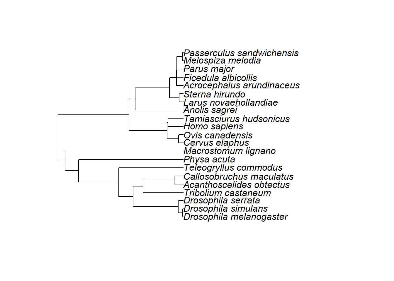
We then checked if the phylogenetic tree had been build correctly.
## CHECK PHYLOGENETIC TREE
sort(RS_theTree$tip.label) == sort(unique(RS_gen_metaData$animal)) # check if tip names correspond to data names
is.ultrametric(RS_theTree) # check if BL are aligned contemporaneously
isSymmetric(vcv(RS_theTree, corr=TRUE)) # check symmetry of phylogenetic correlation matrix
rawC <- vcv(RS_theTree, corr=TRUE)
is.positive.definite(rawC) # if FALSE will have to force symmetry
forcedC <- as.matrix(forceSymmetric(vcv(RS_theTree, corr=TRUE)))
is.positive.definite(forcedC)
comparedC <- rawC == forcedC
rawC[cbind(which(comparedC!=TRUE, arr.ind = T))] - forcedC[cbind(which(comparedC!=TRUE, arr.ind = T))] < 1e-5
Next, we set the priors for the MCMC models using uninformative priors (V = 1, nu = 0.01) and an effective sample size of 20000 (number of iterations = 11000000, burn-in = 1000000, thinning interval = 500). We also set the index and study ID as factors.
## Prior settings, iterations
pr<-list(R=list(V=1,nu=0.01),  G=list(G1=list(V=1,nu=0.01),
                                      G2=list(V=1,nu=0.01),
                                      G3=list(V=1,nu=0.01)))


BURNIN =  1000000
NITT   = 11000000
THIN   =      500


RS_phen_metaData$Index <- as.factor(RS_phen_metaData$Index)
RS_phen_metaData$Study_ID <- as.factor(RS_phen_metaData$Study_ID)
RS_gen_metaData$Index <- as.factor(RS_gen_metaData$Index)
RS_gen_metaData$Study_ID <- as.factor(RS_gen_metaData$Study_ID)
MCMC models for reproductive success
First, we ran the MCMC testing for overall differences in phenotypic variance in reproductive success (‘phenCV’) between males and females (‘Sex’). The model includes the species (‘animal’), estimate ID (‘Index’) and study ID (‘Study_ID’) as random factors (Table 1).
RS_phen_MCMC_model <- MCMCglmm(phenCV~factor(Sex),random=~animal + Index + Study_ID,
                          pedigree=RS_theTree,
                          prior=pr,
                          data=RS_phen_metaData,
                          pr = TRUE, burnin = BURNIN, nitt=NITT, thin=THIN)

summary(RS_phen_MCMC_model)
 Iterations = 1000001:10999501
 Thinning interval  = 500
 Sample size  = 20000

 DIC: 49.23811

 G-structure:  ~animal

       post.mean l-95% CI u-95% CI eff.samp
animal   0.03025 0.001009  0.09079    20000

               ~Index

      post.mean l-95% CI u-95% CI eff.samp
Index   0.05891 0.004482   0.1198    20127

               ~Study_ID

         post.mean  l-95% CI u-95% CI eff.samp
Study_ID    0.0629 0.0009535   0.1457    20000

 R-structure:  ~units

      post.mean l-95% CI u-95% CI eff.samp
units   0.05958  0.04009  0.08303    20000

 Location effects: phenCV ~ factor(Sex)

                       post.mean l-95% CI u-95% CI eff.samp  pMCMC
(Intercept)               0.6940   0.4801   0.9185    20000  2e-04 ***
factor(Sex)phenCV_male    0.2341   0.1502   0.3231    20000 <5e-05 ***
---
Signif. codes:  0 '***' 0.001 '**' 0.01 '*' 0.05 '.' 0.1 ' ' 1
We then expanded the model to include an interaction of mating system (‘Mating_system’) and sex (Supplementary File 1).
RS_phen_MatSyst_MCMC_model <- MCMCglmm(phenCV~factor(Sex) * factor(Mating_system),random=~animal + Index + Study_ID,
                                  pedigree=RS_theTree,
                                  prior=pr,
                                  data=RS_phen_metaData,
                                  pr = TRUE, burnin = BURNIN, nitt=NITT, thin=THIN)

summary(RS_phen_MatSyst_MCMC_model)
 Iterations = 1000001:10999501
 Thinning interval  = 500
 Sample size  = 20000

 DIC: 30.63378

 G-structure:  ~animal

       post.mean l-95% CI u-95% CI eff.samp
animal   0.04896 0.001384   0.1414    20000

               ~Index

      post.mean l-95% CI u-95% CI eff.samp
Index   0.06211 0.007444   0.1213    20000

               ~Study_ID

         post.mean l-95% CI u-95% CI eff.samp
Study_ID   0.05915 0.001256   0.1407    20000

 R-structure:  ~units

      post.mean l-95% CI u-95% CI eff.samp
units   0.05011  0.03313  0.06948    20000

 Location effects: phenCV ~ factor(Sex) * factor(Mating_system)

                                                     post.mean l-95% CI
(Intercept)                                            0.67560  0.28295
factor(Sex)phenCV_male                                -0.01151 -0.17385
factor(Mating_system)polygamy                          0.02515 -0.34242
factor(Sex)phenCV_male:factor(Mating_system)polygamy   0.32320  0.13743
                                                     u-95% CI eff.samp  pMCMC
(Intercept)                                           1.04732    19513 0.0044
factor(Sex)phenCV_male                                0.14407    20698 0.8854
factor(Mating_system)polygamy                         0.40737    20000 0.9133
factor(Sex)phenCV_male:factor(Mating_system)polygamy  0.50448    20433 0.0005

(Intercept)                                          **
factor(Sex)phenCV_male
factor(Mating_system)polygamy
factor(Sex)phenCV_male:factor(Mating_system)polygamy ***
---
Signif. codes:  0 '***' 0.001 '**' 0.01 '*' 0.05 '.' 0.1 ' ' 1
Next, we ran the MCMC models examining the genetic variance in reproductive success (‘genCV’). First, the overall model for a sex difference (Table 1).
RS_gen_MCMC_model <- MCMCglmm(genCV~factor(Sex),random=~animal + Index + Study_ID,
                       pedigree=RS_theTree,
                       prior=pr,
                       data=RS_gen_metaData,
                       pr = TRUE, burnin = BURNIN, nitt=NITT, thin=THIN)
summary(RS_gen_MCMC_model)
 Iterations = 1000001:10999501
 Thinning interval  = 500
 Sample size  = 20000

 DIC: -131.1002

 G-structure:  ~animal

       post.mean l-95% CI u-95% CI eff.samp
animal   0.01675 0.000811  0.04572    20000

               ~Index

      post.mean l-95% CI u-95% CI eff.samp
Index  0.005744 0.001154  0.01197    20000

               ~Study_ID

         post.mean l-95% CI u-95% CI eff.samp
Study_ID    0.0143 0.004079  0.02622    19803

 R-structure:  ~units

      post.mean l-95% CI u-95% CI eff.samp
units   0.01469  0.01008  0.01966    20000

 Location effects: genCV ~ factor(Sex)

                      post.mean l-95% CI u-95% CI eff.samp  pMCMC
(Intercept)             0.25736  0.11555  0.40998    20000 0.0015 **
factor(Sex)genCV_male   0.08653  0.04389  0.12967    20000 0.0002 ***
---
Signif. codes:  0 '***' 0.001 '**' 0.01 '*' 0.05 '.' 0.1 ' ' 1
Secondly, we included an interaction of mating system (‘Mating_system’) and sex (Supplementary File 1).
RS_gen_MatSyst_MCMC_model <- MCMCglmm(genCV~factor(Sex) * factor(Mating_system),random=~animal + Index + Study_ID,
                  pedigree=RS_theTree,
                  prior=pr,
                  data=RS_gen_metaData,
                  pr = TRUE, burnin = BURNIN, nitt=NITT, thin=THIN)
summary(RS_gen_MatSyst_MCMC_model)
 Iterations = 1000001:10999501
 Thinning interval  = 500
 Sample size  = 20000

 DIC: -140.0636

 G-structure:  ~animal

       post.mean  l-95% CI u-95% CI eff.samp
animal   0.01649 0.0009349   0.0464    20108

               ~Index

      post.mean l-95% CI u-95% CI eff.samp
Index   0.00612 0.001243  0.01246    20000

               ~Study_ID

         post.mean l-95% CI u-95% CI eff.samp
Study_ID   0.01475 0.004272  0.02715    20000

 R-structure:  ~units

      post.mean l-95% CI u-95% CI eff.samp
units   0.01336 0.009143  0.01815    20000

 Location effects: genCV ~ factor(Sex) * factor(Mating_system)

                                                    post.mean l-95% CI u-95% CI
(Intercept)                                           0.26415  0.08402  0.46431
factor(Sex)genCV_male                                -0.01501 -0.09852  0.06915
factor(Mating_system)polygamy                        -0.01125 -0.16752  0.14601
factor(Sex)genCV_male:factor(Mating_system)polygamy   0.13382  0.03913  0.23038
                                                    eff.samp  pMCMC
(Intercept)                                            20000 0.0048 **
factor(Sex)genCV_male                                  20000 0.7240
factor(Mating_system)polygamy                          20000 0.8884
factor(Sex)genCV_male:factor(Mating_system)polygamy    20353 0.0084 **
---
Signif. codes:  0 '***' 0.001 '**' 0.01 '*' 0.05 '.' 0.1 ' ' 1
MCMC models for lifespan
In addition to the previous models on reproductive success, ran MCMC models to test for differences in the phenotypic and genetic variances in males and females for lifespan.
First, we pruned the phylogenetic tree to the data subset.
## PRUNE PHYLOGENETIC TREE TO DATA SUBSET
LS_gen_metaData$animal <- factor(LS_gen_metaData$animal)
is.factor(LS_gen_metaData$animal)
LS_Species_Data <- unique(LS_gen_metaData$animal)
summary(LS_Species_Data)
LS_theTree<-drop.tip(theTree, theTree$tip.label[-na.omit(match(LS_Species_Data, theTree$tip.label))])
plot(LS_theTree)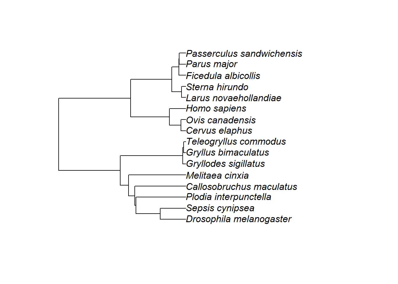
We then checked if the phylogenetic tree had been build correctly.
## CHECK PHYLOGENETIC TREE
sort(LS_theTree$tip.label) == sort(unique(LS_gen_metaData$animal)) # check if tip names correspond to data names
is.ultrametric(LS_theTree) # check if BL are aligned contemporaneously
isSymmetric(vcv(LS_theTree, corr=TRUE)) # check symmetry of phylogenetic correlation matrix
rawC <- vcv(LS_theTree, corr=TRUE)
is.positive.definite(rawC) # if FALSE will have to force symmetry
forcedC <- as.matrix(forceSymmetric(vcv(LS_theTree, corr=TRUE)))
is.positive.definite(forcedC)
comparedC <- rawC == forcedC
rawC[cbind(which(comparedC!=TRUE, arr.ind = T))] - forcedC[cbind(which(comparedC!=TRUE, arr.ind = T))] < 1e-5
Next, we set the priors for the MCMC models using uninformative priors (V = 1, nu = 0.002) and an effective sample size of 20000 (number of iterations = 11000000, burn-in = 1000000, thinning interval = 500). We also set the index and study ID as factors.
## Prior settings, iterations
pr<-list(R=list(V=1,nu=0.01), G=list(G1=list(V=1,nu=0.01),
                                      G2=list(V=1,nu=0.01),
                                      G3=list(V=1,nu=0.01)))

BURNIN =  1000000
NITT   = 11000000
THIN   =      500


LS_phen_metaData$Index <- as.factor(LS_phen_metaData$Index)
LS_phen_metaData$Study_ID <- as.factor(LS_phen_metaData$Study_ID)
LS_gen_metaData$Index <- as.factor(LS_gen_metaData$Index)
LS_gen_metaData$Study_ID <- as.factor(LS_gen_metaData$Study_ID)
First, we ran the MCMC testing for overall differences in phenotypic variance in lifespan (‘phenCV’) between males and females (‘Sex’). The model includes the species (‘animal’), estimate ID (‘Index’) and study ID (‘Study_ID’) as random factors (Table 1).
LS_phen_MCMC_model <- MCMCglmm(phenCV~factor(Sex),random=~animal + Index + Study_ID,
                               pedigree=LS_theTree,
                               prior=pr,
                               data=LS_phen_metaData,
                               pr = TRUE, burnin = BURNIN, nitt=NITT, thin=THIN)

summary(LS_phen_MCMC_model)
 Iterations = 1000001:10999501
 Thinning interval  = 500
 Sample size  = 20000

 DIC: -189.6669

 G-structure:  ~animal

       post.mean l-95% CI u-95% CI eff.samp
animal   0.04176 0.001415   0.1304    18236

               ~Index

      post.mean l-95% CI u-95% CI eff.samp
Index   0.01119 0.002609  0.02341    20620

               ~Study_ID

         post.mean l-95% CI u-95% CI eff.samp
Study_ID   0.02779 0.005106  0.05456    19469

 R-structure:  ~units

      post.mean l-95% CI u-95% CI eff.samp
units   0.00341  0.00201 0.005072    20000

 Location effects: phenCV ~ factor(Sex)

                       post.mean  l-95% CI  u-95% CI eff.samp  pMCMC
(Intercept)             0.430756  0.175653  0.689118    20000 0.0073 **
factor(Sex)phenCV_male -0.004789 -0.030274  0.021496    20000 0.7104
---
Signif. codes:  0 '***' 0.001 '**' 0.01 '*' 0.05 '.' 0.1 ' ' 1
We then expanded the model to include an interaction of mating system (‘Mating_system’) and sex (Supplementary File 1).
LS_phen_MatSyst_MCMC_model <- MCMCglmm(phenCV~factor(Sex) * factor(Mating_system),random=~animal + Index + Study_ID,
                                       pedigree=LS_theTree,
                                       prior=pr,
                                       data=LS_phen_metaData,
                                       pr = TRUE, burnin = BURNIN, nitt=NITT, thin=THIN)

summary(LS_phen_MatSyst_MCMC_model)
 Iterations = 1000001:10999501
 Thinning interval  = 500
 Sample size  = 20000

 DIC: -190.3721

 G-structure:  ~animal

       post.mean  l-95% CI u-95% CI eff.samp
animal   0.06899 0.0007289   0.2345    20000

               ~Index

      post.mean l-95% CI u-95% CI eff.samp
Index   0.01096 0.002546   0.0227    20000

               ~Study_ID

         post.mean l-95% CI u-95% CI eff.samp
Study_ID   0.02674 0.003981  0.05366    20000

 R-structure:  ~units

      post.mean l-95% CI u-95% CI eff.samp
units   0.00334 0.001979 0.005002    20000

 Location effects: phenCV ~ factor(Sex) * factor(Mating_system)

                                                     post.mean l-95% CI
(Intercept)                                            0.35987 -0.04926
factor(Sex)phenCV_male                                 0.02678 -0.02719
factor(Mating_system)polygamy                          0.10169 -0.22019
factor(Sex)phenCV_male:factor(Mating_system)polygamy  -0.04085 -0.10084
                                                     u-95% CI eff.samp  pMCMC
(Intercept)                                           0.72282    20000 0.0871 .
factor(Sex)phenCV_male                                0.07867    19197 0.3186
factor(Mating_system)polygamy                         0.43592    20000 0.5719
factor(Sex)phenCV_male:factor(Mating_system)polygamy  0.02066    19512 0.1834
---
Signif. codes:  0 '***' 0.001 '**' 0.01 '*' 0.05 '.' 0.1 ' ' 1
Next, we ran the MCMC models examining the genetic variance in lifespan (‘genCV’). First, the overall model for a sex difference (Table 1).
LS_gen_MCMC_model <- MCMCglmm(genCV~factor(Sex),random=~animal + Index + Study_ID,
                              pedigree=LS_theTree,
                              prior=pr,
                              data=LS_gen_metaData,
                              pr = TRUE, burnin = BURNIN, nitt=NITT, thin=THIN)
summary(LS_gen_MCMC_model)
 Iterations = 1000001:10999501
 Thinning interval  = 500
 Sample size  = 20000

 DIC: -214.4485

 G-structure:  ~animal

       post.mean  l-95% CI u-95% CI eff.samp
animal   0.01277 0.0009457   0.0359    20000

               ~Index

      post.mean  l-95% CI u-95% CI eff.samp
Index  0.002128 0.0006209  0.00431    20000

               ~Study_ID

         post.mean l-95% CI u-95% CI eff.samp
Study_ID   0.00633 0.001698  0.01227    20000

 R-structure:  ~units

      post.mean l-95% CI u-95% CI eff.samp
units  0.002644 0.001612  0.00378    20000

 Location effects: genCV ~ factor(Sex)

                      post.mean  l-95% CI  u-95% CI eff.samp  pMCMC
(Intercept)            0.140077 -0.002497  0.281642    20542 0.0529 .
factor(Sex)genCV_male  0.016722 -0.005430  0.040323    20000 0.1464
---
Signif. codes:  0 '***' 0.001 '**' 0.01 '*' 0.05 '.' 0.1 ' ' 1
Secondly, including an interaction of mating system (‘Mating_system’) and sex (Supplementary File 1).
LS_gen_MatSyst_MCMC_model <- MCMCglmm(genCV~factor(Sex) * factor(Mating_system),random=~animal + Index + Study_ID,
                                      pedigree=LS_theTree,
                                      prior=pr,
                                      data=LS_gen_metaData,
                                      pr = TRUE, burnin = BURNIN, nitt=NITT, thin=THIN)
summary(LS_gen_MatSyst_MCMC_model)
 Iterations = 1000001:10999501
 Thinning interval  = 500
 Sample size  = 20000

 DIC: -216.0559

 G-structure:  ~animal

       post.mean  l-95% CI u-95% CI eff.samp
animal   0.01274 0.0009163  0.03568    20000

               ~Index

      post.mean  l-95% CI u-95% CI eff.samp
Index   0.00212 0.0005475  0.00422    20000

               ~Study_ID

         post.mean l-95% CI u-95% CI eff.samp
Study_ID  0.006334 0.001703   0.0122    19491

 R-structure:  ~units

      post.mean l-95% CI u-95% CI eff.samp
units   0.00256 0.001542 0.003665    20000

 Location effects: genCV ~ factor(Sex) * factor(Mating_system)

                                                    post.mean  l-95% CI
(Intercept)                                          0.162764  0.001801
factor(Sex)genCV_male                                0.049759  0.003971
factor(Mating_system)polygamy                       -0.035428 -0.162993
factor(Sex)genCV_male:factor(Mating_system)polygamy -0.042970 -0.095263
                                                     u-95% CI eff.samp  pMCMC
(Intercept)                                          0.329991    20000 0.0538 .
factor(Sex)genCV_male                                0.097362    19913 0.0391 *
factor(Mating_system)polygamy                        0.098228    20000 0.5792
factor(Sex)genCV_male:factor(Mating_system)polygamy  0.011890    19298 0.1159
---
Signif. codes:  0 '***' 0.001 '**' 0.01 '*' 0.05 '.' 0.1 ' ' 1
Subsetting data by mating system
We then analysed the data separately for socially monogamous and polygamous species.
First we subset the data into socially monogamous and polygamous species for all fitness categories (lifespan and reproductive success) and their phenotypic as well as genetic variances.
## Additional subsetting
RS_gen_Monogamy_metaData<-subset(RS_gen_metaData, Mating_system == "monogamy")
RS_gen_Polygamy_metaData<-subset(RS_gen_metaData, Mating_system == "polygamy")

RS_phen_Monogamy_metaData<-subset(RS_phen_metaData, Mating_system == "monogamy")
RS_phen_Polygamy_metaData<-subset(RS_phen_metaData, Mating_system == "polygamy")

LS_gen_Monogamy_metaData<-subset(LS_gen_metaData, Mating_system == "monogamy")
LS_gen_Polygamy_metaData<-subset(LS_gen_metaData, Mating_system == "polygamy")

LS_phen_Monogamy_metaData<-subset(LS_phen_metaData, Mating_system == "monogamy")
LS_phen_Polygamy_metaData<-subset(LS_phen_metaData, Mating_system == "polygamy")
We then pruned the phylogenetic tree to all species with data on lifespan or reproductive success for monogamous and polygamous species separately.
## PRUNE PHYLOGENETIC TREES
RS_gen_Monogamy_metaData$animal <- factor(RS_gen_Monogamy_metaData$animal)
RS_Monogamy_Species_Data <- unique(RS_gen_Monogamy_metaData$animal)
summary(RS_Monogamy_Species_Data)
RS_Monogamy_theTree<-drop.tip(theTree, theTree$tip.label[-na.omit(match(RS_Monogamy_Species_Data, theTree$tip.label))])
plot(RS_Monogamy_theTree)RS_gen_Polygamy_metaData$animal <- factor(RS_gen_Polygamy_metaData$animal)
RS_Polygamy_Species_Data <- unique(RS_gen_Polygamy_metaData$animal)
summary(RS_Polygamy_Species_Data)
RS_Polygamy_theTree<-drop.tip(theTree, theTree$tip.label[-na.omit(match(RS_Polygamy_Species_Data, theTree$tip.label))])
plot(RS_Polygamy_theTree)LS_gen_Monogamy_metaData$animal <- factor(LS_gen_Monogamy_metaData$animal)
LS_Monogamy_Species_Data <- unique(LS_gen_Monogamy_metaData$animal)
summary(LS_Monogamy_Species_Data)
LS_Monogamy_theTree<-drop.tip(theTree, theTree$tip.label[-na.omit(match(LS_Monogamy_Species_Data, theTree$tip.label))])
plot(LS_Monogamy_theTree)LS_gen_Polygamy_metaData$animal <- factor(LS_gen_Polygamy_metaData$animal)
LS_Polygamy_Species_Data <- unique(LS_gen_Polygamy_metaData$animal)
summary(LS_Polygamy_Species_Data)
LS_Polygamy_theTree<-drop.tip(theTree, theTree$tip.label[-na.omit(match(LS_Polygamy_Species_Data, theTree$tip.label))])
plot(LS_Polygamy_theTree)MCMCs for reproductive success
We then ran the MCMC models, first for the phenotypic variance in reproductive success in monogamous species (Table 1).
RS_phen_Monogamy_MCMC_model <- MCMCglmm(phenCV~factor(Sex),random=~animal + Index + Study_ID,
                               pedigree=RS_Monogamy_theTree,
                               prior=pr,
                               data=RS_phen_Monogamy_metaData,
                               pr = TRUE, burnin = BURNIN, nitt=NITT, thin=THIN)
summary(RS_phen_Monogamy_MCMC_model)
 Iterations = 1000001:10999501
 Thinning interval  = 500
 Sample size  = 20000

 DIC: -65.819

 G-structure:  ~animal

       post.mean  l-95% CI u-95% CI eff.samp
animal    0.5285 0.0008104    2.457    20466

               ~Index

      post.mean  l-95% CI u-95% CI eff.samp
Index   0.09383 0.0008326   0.2588    19526

               ~Study_ID

         post.mean  l-95% CI u-95% CI eff.samp
Study_ID   0.09331 0.0009878   0.2594    20310

 R-structure:  ~units

      post.mean l-95% CI u-95% CI eff.samp
units  0.004682 0.001673 0.008786    20000

 Location effects: phenCV ~ factor(Sex)

                       post.mean l-95% CI u-95% CI eff.samp  pMCMC
(Intercept)              0.85145 -0.11209  1.84827    19853 0.0696 .
factor(Sex)phenCV_male  -0.01228 -0.06019  0.03900    20000 0.5982
---
Signif. codes:  0 '***' 0.001 '**' 0.01 '*' 0.05 '.' 0.1 ' ' 1
Next, we ran the MCMC model for the genetic variance in reproductive success in monogamous species (Table 1).
RS_gen_Monogamy_MCMC_model <- MCMCglmm(genCV~factor(Sex),random=~animal + Index + Study_ID,
                                        pedigree=RS_Monogamy_theTree,
                                        prior=pr,
                                        data=RS_gen_Monogamy_metaData,
                                       pr = TRUE, burnin = BURNIN, nitt=NITT, thin=THIN)
summary(RS_gen_Monogamy_MCMC_model)
 Iterations = 1000001:10999501
 Thinning interval  = 500
 Sample size  = 20000

 DIC: -51.50387

 G-structure:  ~animal

       post.mean  l-95% CI u-95% CI eff.samp
animal    0.0603 0.0006262   0.2358    20000

               ~Index

      post.mean l-95% CI u-95% CI eff.samp
Index   0.01264 0.001037  0.03208    20000

               ~Study_ID

         post.mean  l-95% CI u-95% CI eff.samp
Study_ID   0.01264 0.0009578  0.03221    20000

 R-structure:  ~units

      post.mean l-95% CI u-95% CI eff.samp
units  0.007524 0.002912  0.01365    20000

 Location effects: genCV ~ factor(Sex)

                      post.mean l-95% CI u-95% CI eff.samp pMCMC
(Intercept)             0.21237 -0.13103  0.53680    20533 0.125
factor(Sex)genCV_male  -0.01467 -0.07633  0.04813    20000 0.624
Then followed the models for reproductive success in polygamous species. First, the MCMC for the phenotypic variance in reproductive success in polygamous species (Table 1).
RS_phen_Polygamy_MCMC_model <- MCMCglmm(phenCV~factor(Sex),random=~animal + Index + Study_ID,
                                        pedigree=RS_Polygamy_theTree,
                                        prior=pr,
                                        data=RS_phen_Polygamy_metaData,
                                        pr = TRUE, burnin = BURNIN, nitt=NITT, thin=THIN)
summary(RS_phen_Polygamy_MCMC_model)
 Iterations = 1000001:10999501
 Thinning interval  = 500
 Sample size  = 20000

 DIC: 43.71919

 G-structure:  ~animal

       post.mean  l-95% CI u-95% CI eff.samp
animal   0.05677 0.0009819   0.1682    20561

               ~Index

      post.mean l-95% CI u-95% CI eff.samp
Index   0.05064 0.002271   0.1065    19507

               ~Study_ID

         post.mean l-95% CI u-95% CI eff.samp
Study_ID   0.05453 0.001008    0.142    20293

 R-structure:  ~units

      post.mean l-95% CI u-95% CI eff.samp
units   0.06591  0.04087  0.09548    20000

 Location effects: phenCV ~ factor(Sex)

                       post.mean l-95% CI u-95% CI eff.samp  pMCMC
(Intercept)               0.7011   0.4155   0.9878    20000  4e-04 ***
factor(Sex)phenCV_male    0.3121   0.2116   0.4210    20000 <5e-05 ***
---
Signif. codes:  0 '***' 0.001 '**' 0.01 '*' 0.05 '.' 0.1 ' ' 1
Next, we ran the MCMC model for the genetic variance in reproductive success in polygamous species (Table 1).
RS_gen_Polygamy_MCMC_model <- MCMCglmm(genCV~factor(Sex),random=~animal + Index + Study_ID,
                                       pedigree=RS_Polygamy_theTree,
                                       prior=pr,
                                       data=RS_gen_Polygamy_metaData,
                                       pr = TRUE, burnin = BURNIN, nitt=NITT, thin=THIN)
summary(RS_gen_Polygamy_MCMC_model)
 Iterations = 1000001:10999501
 Thinning interval  = 500
 Sample size  = 20000

 DIC: -95.4313

 G-structure:  ~animal

       post.mean  l-95% CI u-95% CI eff.samp
animal   0.01739 0.0008811   0.0504    20000

               ~Index

      post.mean l-95% CI u-95% CI eff.samp
Index  0.006173 0.001135  0.01314    19406

               ~Study_ID

         post.mean l-95% CI u-95% CI eff.samp
Study_ID   0.01805 0.004008  0.03502    20000

 R-structure:  ~units

      post.mean l-95% CI u-95% CI eff.samp
units   0.01545 0.009833  0.02132    19382

 Location effects: genCV ~ factor(Sex)

                      post.mean l-95% CI u-95% CI eff.samp  pMCMC
(Intercept)             0.25194  0.09535  0.41043    20000 0.0053 **
factor(Sex)genCV_male   0.11857  0.06907  0.16870    20000 <5e-05 ***
---
Signif. codes:  0 '***' 0.001 '**' 0.01 '*' 0.05 '.' 0.1 ' ' 1
MCMCs for lifespan
Now followed the mating system specific MCMCs for lifespan. We first ran the MCMC models for the phenotypic variance in lifespan in monogamous species (Table 1).
LS_phen_Monogamy_MCMC_model <- MCMCglmm(phenCV~factor(Sex),random=~animal + Index + Study_ID,
                                        pedigree=LS_Monogamy_theTree,
                                        prior=pr,
                                        data=LS_phen_Monogamy_metaData,
                                        pr = TRUE, burnin = BURNIN, nitt=NITT, thin=THIN)
summary(LS_phen_Monogamy_MCMC_model)
 Iterations = 1000001:10999501
 Thinning interval  = 500
 Sample size  = 20000

 DIC: -51.18382

 G-structure:  ~animal

       post.mean  l-95% CI u-95% CI eff.samp
animal   0.08956 0.0006984   0.3387    20000

               ~Index

      post.mean  l-95% CI u-95% CI eff.samp
Index   0.03274 0.0009689   0.0942    20000

               ~Study_ID

         post.mean l-95% CI u-95% CI eff.samp
Study_ID   0.03255 0.001071  0.09425    20000

 R-structure:  ~units

      post.mean  l-95% CI u-95% CI eff.samp
units  0.003234 0.0007601 0.007181    20000

 Location effects: phenCV ~ factor(Sex)

                       post.mean l-95% CI u-95% CI eff.samp pMCMC
(Intercept)              0.51524  0.10435  0.91095    20000 0.028 *
factor(Sex)phenCV_male   0.02670 -0.02984  0.07817    20000 0.286
---
Signif. codes:  0 '***' 0.001 '**' 0.01 '*' 0.05 '.' 0.1 ' ' 1
Next, we ran the MCMC model for the genetic variance in lifespan in monogamous species (Table 1).
LS_gen_Monogamy_MCMC_model <- MCMCglmm(genCV~factor(Sex),random=~animal + Index + Study_ID,
                                       pedigree=LS_Monogamy_theTree,
                                       prior=pr,
                                       data=LS_gen_Monogamy_metaData,
                                       pr = TRUE, burnin = BURNIN, nitt=NITT, thin=THIN)
summary(LS_gen_Monogamy_MCMC_model)
 Iterations = 1000001:10999501
 Thinning interval  = 500
 Sample size  = 20000

 DIC: -35.09093

 G-structure:  ~animal

       post.mean l-95% CI u-95% CI eff.samp
animal   0.05535 0.001091   0.1965    20000

               ~Index

      post.mean  l-95% CI u-95% CI eff.samp
Index   0.01318 0.0007922  0.03887    20000

               ~Study_ID

         post.mean  l-95% CI u-95% CI eff.samp
Study_ID   0.01314 0.0008344  0.03826    16829

 R-structure:  ~units

      post.mean l-95% CI u-95% CI eff.samp
units  0.006671 0.001822  0.01405    20000

 Location effects: genCV ~ factor(Sex)

                      post.mean l-95% CI u-95% CI eff.samp pMCMC
(Intercept)             0.14569 -0.19152  0.47027    20000 0.261
factor(Sex)genCV_male   0.05010 -0.02676  0.12622    20000 0.174
Then followed the models for lifespan in polygamous species. First, the MCMC for the phenotypic variance in lifespan in polygamous species (Table 1).
LS_phen_Polygamy_MCMC_model <- MCMCglmm(phenCV~factor(Sex),random=~animal + Index + Study_ID,
                                        pedigree=LS_Polygamy_theTree,
                                        prior=pr,
                                        data=LS_phen_Polygamy_metaData,
                                        pr = TRUE, burnin = BURNIN, nitt=NITT, thin=THIN)
summary(LS_phen_Polygamy_MCMC_model)
 Iterations = 1000001:10999501
 Thinning interval  = 500
 Sample size  = 20000

 DIC: -138.2843

 G-structure:  ~animal

       post.mean l-95% CI u-95% CI eff.samp
animal    0.1165 0.001366    0.319    20000

               ~Index

      post.mean l-95% CI u-95% CI eff.samp
Index  0.009194 0.002231    0.019    20000

               ~Study_ID

         post.mean l-95% CI u-95% CI eff.samp
Study_ID   0.01863 0.002682  0.04381    20000

 R-structure:  ~units

      post.mean l-95% CI u-95% CI eff.samp
units  0.003992 0.002064 0.006217    20000

 Location effects: phenCV ~ factor(Sex)

                       post.mean l-95% CI u-95% CI eff.samp  pMCMC
(Intercept)              0.50253  0.09672  0.93815    20000 0.0206 *
factor(Sex)phenCV_male  -0.01390 -0.04549  0.01817    20000 0.3933
---
Signif. codes:  0 '***' 0.001 '**' 0.01 '*' 0.05 '.' 0.1 ' ' 1
Next, we run the MCMC model for the genetic variance in lifespan in polygamous species (Table 1).
LS_gen_Polygamy_MCMC_model <- MCMCglmm(genCV~factor(Sex),random=~animal + Index + Study_ID,
                                       pedigree=LS_Polygamy_theTree,
                                       prior=pr,
                                       data=LS_gen_Polygamy_metaData,
                                       pr = TRUE, burnin = BURNIN, nitt=NITT, thin=THIN)
summary(LS_gen_Polygamy_MCMC_model)
 Iterations = 1000001:10999501
 Thinning interval  = 500
 Sample size  = 20000

 DIC: -180.7517

 G-structure:  ~animal

       post.mean  l-95% CI u-95% CI eff.samp
animal  0.009475 0.0007683  0.02627    20000

               ~Index

      post.mean  l-95% CI u-95% CI eff.samp
Index  0.001933 0.0006136 0.003849    20000

               ~Study_ID

         post.mean l-95% CI u-95% CI eff.samp
Study_ID  0.005425 0.001315   0.0111    20000

 R-structure:  ~units

      post.mean l-95% CI u-95% CI eff.samp
units  0.002116 0.001202 0.003159    20000

 Location effects: genCV ~ factor(Sex)

                      post.mean  l-95% CI  u-95% CI eff.samp  pMCMC
(Intercept)            0.132430  0.012503  0.267101    20757 0.0401 *
factor(Sex)genCV_male  0.006762 -0.017139  0.029570    20000 0.5576
---
Signif. codes:  0 '***' 0.001 '**' 0.01 '*' 0.05 '.' 0.1 ' ' 1
Analyses of vertebrates
In this part, we analysed the vertebrate species separately, as all monogamous species in this dataset are vertebrates (see Supplementary Files 2 & 3).
We first subset our data frame to only include vertebrates (mammalia, aves or reptilia).
Data_vertebrates <-subset(Data, Class == "Mammalia" | Class == "Aves" | Class == "Reptilia")

stacked_gen_Data_vertebrates <- gather(Data_vertebrates, key = "Sex",value = "genCV", genCV_male, genCV_female)
stacked_phen_Data_vertebrates <- gather(Data_vertebrates, key = "Sex",value = "phenCV", phenCV_male, phenCV_female)


RS_gen_metaData_vertebrates<-subset(stacked_gen_Data_vertebrates, FitnessCat == "RS")
LS_gen_metaData_vertebrates<-subset(stacked_gen_Data_vertebrates, FitnessCat == "LS")

RS_phen_metaData_vertebrates<-subset(stacked_phen_Data_vertebrates, FitnessCat == "RS")
LS_phen_metaData_vertebrates<-subset(stacked_phen_Data_vertebrates, FitnessCat == "LS")
MCMCs for reproductive success
We pruned the phylogenetic tree to all vertebrate species with data on reproductive success.
## PRUNE PHYLOGENETIC TREE TO DATA SUBSET
RS_gen_metaData_vertebrates$animal <- factor(RS_gen_metaData_vertebrates$animal)
is.factor(RS_gen_metaData_vertebrates$animal)
RS_Species_Data_vertebrates <- unique(RS_gen_metaData_vertebrates$animal)
summary(RS_Species_Data_vertebrates)
RS_theTree_vertebrates<-drop.tip(theTree, theTree$tip.label[-na.omit(match(RS_Species_Data_vertebrates, theTree$tip.label))])
plot(RS_theTree_vertebrates)RS_phen_metaData_vertebrates$Index <- as.factor(RS_phen_metaData_vertebrates$Index)
RS_phen_metaData_vertebrates$Study_ID <- as.factor(RS_phen_metaData_vertebrates$Study_ID)
RS_gen_metaData_vertebrates$Index <- as.factor(RS_gen_metaData_vertebrates$Index)
RS_gen_metaData_vertebrates$Study_ID <- as.factor(RS_gen_metaData_vertebrates$Study_ID)We then first ran the MCMC models for the phenotypic variance in reproductive success in vertebrate species (Supplementary File 2).
RS_phen_MCMC_model_vertebrates <- MCMCglmm(phenCV~factor(Sex),random=~animal + Index + Study_ID,
                               pedigree=RS_theTree,
                               prior=pr,
                               data=RS_phen_metaData_vertebrates,
                               pr = TRUE, burnin = BURNIN, nitt=NITT, thin=THIN)
summary(RS_phen_MCMC_model_vertebrates)
 Iterations = 1000001:10999501
 Thinning interval  = 500
 Sample size  = 20000

 DIC: 37.24732

 G-structure:  ~animal

       post.mean  l-95% CI u-95% CI eff.samp
animal   0.09917 0.0008523   0.3995    20636

               ~Index

      post.mean l-95% CI u-95% CI eff.samp
Index   0.09962 0.001261   0.2648    20000

               ~Study_ID

         post.mean l-95% CI u-95% CI eff.samp
Study_ID   0.09915 0.001095   0.2611    20000

 R-structure:  ~units

      post.mean l-95% CI u-95% CI eff.samp
units   0.09002  0.04239   0.1505    21306

 Location effects: phenCV ~ factor(Sex)

                       post.mean l-95% CI u-95% CI eff.samp  pMCMC
(Intercept)              0.86708  0.28132  1.45441    18529 0.0176 *
factor(Sex)phenCV_male   0.18751  0.01349  0.35834    20000 0.0345 *
---
Signif. codes:  0 '***' 0.001 '**' 0.01 '*' 0.05 '.' 0.1 ' ' 1
Next, we ran the MCMC model for the phenotypic variance in reproductive success in vertebrate species including an interaction of mating system (‘Mating_system’) and sex (Supplementary File 3).
RS_phen_MatSyst_MCMC_model_vertebrates <- MCMCglmm(phenCV~factor(Sex) * factor(Mating_system),random=~animal + Index + Study_ID,
                                       pedigree=RS_theTree,
                                       prior=pr,
                                       data=RS_phen_metaData_vertebrates,
                                       pr = TRUE, burnin = BURNIN, nitt=NITT, thin=THIN)
summary(RS_phen_MatSyst_MCMC_model_vertebrates)
 Iterations = 1000001:10999501
 Thinning interval  = 500
 Sample size  = 20000

 DIC: 11.11587

 G-structure:  ~animal

       post.mean  l-95% CI u-95% CI eff.samp
animal    0.1391 0.0007481   0.5509    20000

               ~Index

      post.mean l-95% CI u-95% CI eff.samp
Index     0.102 0.001107    0.265    20000

               ~Study_ID

         post.mean l-95% CI u-95% CI eff.samp
Study_ID    0.1029 0.001023   0.2648    20000

 R-structure:  ~units

      post.mean l-95% CI u-95% CI eff.samp
units   0.04825  0.02307  0.08173    20000

 Location effects: phenCV ~ factor(Sex) * factor(Mating_system)

                                                     post.mean l-95% CI
(Intercept)                                            0.83082  0.12727
factor(Sex)phenCV_male                                -0.01322 -0.17314
factor(Mating_system)polygamy                          0.05426 -0.43032
factor(Sex)phenCV_male:factor(Mating_system)polygamy   0.57623  0.31328
                                                     u-95% CI eff.samp  pMCMC
(Intercept)                                           1.49595    20000 0.0366
factor(Sex)phenCV_male                                0.14936    20000 0.8575
factor(Mating_system)polygamy                         0.54381    20000 0.8275
factor(Sex)phenCV_male:factor(Mating_system)polygamy  0.85478    20000 0.0005

(Intercept)                                          *
factor(Sex)phenCV_male
factor(Mating_system)polygamy
factor(Sex)phenCV_male:factor(Mating_system)polygamy ***
---
Signif. codes:  0 '***' 0.001 '**' 0.01 '*' 0.05 '.' 0.1 ' ' 1
Then we ran the MCMC models for the genetic variance in reproductive success in vertebrate species (Supplementary File 2).
RS_gen_MCMC_model_vertebrates <- MCMCglmm(genCV~factor(Sex),random=~animal + Index + Study_ID,
                              pedigree=RS_theTree,
                              prior=pr,
                              data=RS_gen_metaData_vertebrates,
                              pr = TRUE, burnin = BURNIN, nitt=NITT, thin=THIN)
summary(RS_gen_MCMC_model_vertebrates)
 Iterations = 1000001:10999501
 Thinning interval  = 500
 Sample size  = 20000

 DIC: -33.89924

 G-structure:  ~animal

       post.mean  l-95% CI u-95% CI eff.samp
animal   0.03326 0.0008146   0.1174    20000

               ~Index

      post.mean l-95% CI u-95% CI eff.samp
Index   0.01177 0.001017  0.02845    20000

               ~Study_ID

         post.mean l-95% CI u-95% CI eff.samp
Study_ID   0.01181 0.001018  0.02876    20453

 R-structure:  ~units

      post.mean l-95% CI u-95% CI eff.samp
units   0.02015   0.0101  0.03242    20000

 Location effects: genCV ~ factor(Sex)

                      post.mean  l-95% CI  u-95% CI eff.samp  pMCMC
(Intercept)            0.178203 -0.133438  0.511197    20749 0.1796
factor(Sex)genCV_male  0.084344  0.003013  0.167764    20000 0.0458 *
---
Signif. codes:  0 '***' 0.001 '**' 0.01 '*' 0.05 '.' 0.1 ' ' 1
Next, we run the MCMC model for the genetic variance in reproductive success in vertebrate species including an interaction of mating system (‘Mating_system’) and sex (Supplementary File 3).
RS_gen_MatSyst_MCMC_model_vertebrates <- MCMCglmm(genCV~factor(Sex) * factor(Mating_system),random=~animal + Index + Study_ID,
                                      pedigree=RS_theTree,
                                      prior=pr,
                                      data=RS_gen_metaData_vertebrates,
                                      pr = TRUE, burnin = BURNIN, nitt=NITT, thin=THIN)
summary(RS_gen_MatSyst_MCMC_model_vertebrates)
 Iterations = 1000001:10999501
 Thinning interval  = 500
 Sample size  = 20000

 DIC: -58.96858

 G-structure:  ~animal

       post.mean  l-95% CI u-95% CI eff.samp
animal   0.03997 0.0006986   0.1471    20000

               ~Index

      post.mean l-95% CI u-95% CI eff.samp
Index   0.01375 0.001176  0.03242    20000

               ~Study_ID

         post.mean l-95% CI u-95% CI eff.samp
Study_ID   0.01386 0.001234  0.03276    19031

 R-structure:  ~units

      post.mean l-95% CI u-95% CI eff.samp
units   0.01093 0.005139  0.01794    19572

 Location effects: genCV ~ factor(Sex) * factor(Mating_system)

                                                    post.mean l-95% CI u-95% CI
(Intercept)                                           0.21437 -0.14739  0.57569
factor(Sex)genCV_male                                -0.01488 -0.09030  0.06004
factor(Mating_system)polygamy                        -0.10892 -0.30136  0.08809
factor(Sex)genCV_male:factor(Mating_system)polygamy   0.28480  0.15776  0.41318
                                                    eff.samp  pMCMC
(Intercept)                                            20000 0.1553
factor(Sex)genCV_male                                  19179 0.6859
factor(Mating_system)polygamy                          20000 0.2653
factor(Sex)genCV_male:factor(Mating_system)polygamy    20000 0.0002 ***
---
Signif. codes:  0 '***' 0.001 '**' 0.01 '*' 0.05 '.' 0.1 ' ' 1
MCMCs for lifespan
Now followed the vertebrate specific MCMCs for lifespan. We pruned the phylogenetic tree to all vertebrate species with data on lifespan.
## PRUNE PHYLOGENETIC TREE TO DATA SUBSET
LS_gen_metaData_vertebrates$animal <- factor(LS_gen_metaData_vertebrates$animal)
is.factor(LS_gen_metaData_vertebrates$animal)
LS_Species_Data_vertebrates <- unique(LS_gen_metaData_vertebrates$animal)
summary(LS_Species_Data_vertebrates)
LS_theTree_vertebrates<-drop.tip(theTree, theTree$tip.label[-na.omit(match(LS_Species_Data_vertebrates, theTree$tip.label))])
plot(LS_theTree_vertebrates)LS_phen_metaData_vertebrates$Index <- as.factor(LS_phen_metaData_vertebrates$Index)
LS_phen_metaData_vertebrates$Study_ID <- as.factor(LS_phen_metaData_vertebrates$Study_ID)
LS_gen_metaData_vertebrates$Index <- as.factor(LS_gen_metaData_vertebrates$Index)
LS_gen_metaData_vertebrates$Study_ID <- as.factor(LS_gen_metaData_vertebrates$Study_ID)We then ran the MCMC models, first for the phenotypic variance in lifespan in vertebrate species (Supplementary File 2).
LS_phen_MCMC_model_vertebrates <- MCMCglmm(phenCV~factor(Sex),random=~animal + Index + Study_ID,
                                           pedigree=LS_theTree,
                                           prior=pr,
                                           data=LS_phen_metaData_vertebrates,
                                           pr = TRUE, burnin = BURNIN, nitt=NITT, thin=THIN)
summary(LS_phen_MCMC_model_vertebrates)
 Iterations = 1000001:10999501
 Thinning interval  = 500
 Sample size  = 20000

 DIC: -65.06646

 G-structure:  ~animal

       post.mean  l-95% CI u-95% CI eff.samp
animal    0.1863 0.0008099   0.8199    20000

               ~Index

      post.mean  l-95% CI u-95% CI eff.samp
Index   0.04021 0.0009848   0.1085    20000

               ~Study_ID

         post.mean  l-95% CI u-95% CI eff.samp
Study_ID   0.04051 0.0008569   0.1119    20000

 R-structure:  ~units

      post.mean l-95% CI u-95% CI eff.samp
units  0.003681 0.001224 0.007095    21065

 Location effects: phenCV ~ factor(Sex)

                       post.mean  l-95% CI  u-95% CI eff.samp  pMCMC
(Intercept)             0.549536 -0.201479  1.336565    20504 0.0953 .
factor(Sex)phenCV_male -0.003234 -0.049740  0.043387    20000 0.8842
---
Signif. codes:  0 '***' 0.001 '**' 0.01 '*' 0.05 '.' 0.1 ' ' 1
Next, we ran the MCMC model for the phenotypic variance in lifespan in vertebrate species including an interaction of mating system (‘Mating_system’) and sex (Supplementary File 3).
LS_phen_MatSyst_MCMC_model_vertebrates <- MCMCglmm(phenCV~factor(Sex) * factor(Mating_system),random=~animal + Index + Study_ID,
                                                   pedigree=LS_theTree,
                                                   prior=pr,
                                                   data=LS_phen_metaData_vertebrates,
                                                   pr = TRUE, burnin = BURNIN, nitt=NITT, thin=THIN)
summary(LS_phen_MatSyst_MCMC_model_vertebrates)
 Iterations = 1000001:10999501
 Thinning interval  = 500
 Sample size  = 20000

 DIC: -74.97083

 G-structure:  ~animal

       post.mean  l-95% CI u-95% CI eff.samp
animal    0.3496 0.0007483    1.387    20000

               ~Index

      post.mean l-95% CI u-95% CI eff.samp
Index   0.03932 0.000838   0.1129    20000

               ~Study_ID

         post.mean  l-95% CI u-95% CI eff.samp
Study_ID    0.0386 0.0009624   0.1104    20000

 R-structure:  ~units

      post.mean  l-95% CI u-95% CI eff.samp
units   0.00262 0.0008446 0.005217    20000

 Location effects: phenCV ~ factor(Sex) * factor(Mating_system)

                                                     post.mean l-95% CI
(Intercept)                                            0.46957 -0.66281
factor(Sex)phenCV_male                                 0.02686 -0.01946
factor(Mating_system)polygamy                          0.23259 -0.28535
factor(Sex)phenCV_male:factor(Mating_system)polygamy  -0.09772 -0.18490
                                                     u-95% CI eff.samp  pMCMC
(Intercept)                                           1.47749    20425 0.2232
factor(Sex)phenCV_male                                0.07562    20000 0.2382
factor(Mating_system)polygamy                         0.74345    20000 0.3333
factor(Sex)phenCV_male:factor(Mating_system)polygamy -0.01288    20000 0.0307 *
---
Signif. codes:  0 '***' 0.001 '**' 0.01 '*' 0.05 '.' 0.1 ' ' 1
Then we ran the MCMC models for the genetic variance in lifespan in vertebrate species (Supplementary File 2).
LS_gen_MCMC_model_vertebrates <- MCMCglmm(genCV~factor(Sex),random=~animal + Index + Study_ID,
                                          pedigree=LS_theTree,
                                          prior=pr,
                                          data=LS_gen_metaData_vertebrates,
                                          pr = TRUE, burnin = BURNIN, nitt=NITT, thin=THIN)
summary(LS_gen_MCMC_model_vertebrates)
 Iterations = 1000001:10999501
 Thinning interval  = 500
 Sample size  = 20000

 DIC: -48.87279

 G-structure:  ~animal

       post.mean  l-95% CI u-95% CI eff.samp
animal   0.05246 0.0008486    0.183    20000

               ~Index

      post.mean  l-95% CI u-95% CI eff.samp
Index  0.009012 0.0009802  0.02369    20000

               ~Study_ID

         post.mean  l-95% CI u-95% CI eff.samp
Study_ID  0.008917 0.0008867  0.02314    19646

 R-structure:  ~units

      post.mean l-95% CI u-95% CI eff.samp
units  0.006555 0.002279  0.01211    20000

 Location effects: genCV ~ factor(Sex)

                      post.mean l-95% CI u-95% CI eff.samp pMCMC
(Intercept)             0.12917 -0.28251  0.54413    20451 0.376
factor(Sex)genCV_male   0.02424 -0.03988  0.08738    20000 0.421
Next, we ran the MCMC model for the genetic variance in lifespan in vertebrate species including an interaction of mating system (‘Mating_system’) and sex (Supplementary File 3).
LS_gen_MatSyst_MCMC_model_vertebrates <- MCMCglmm(genCV~factor(Sex) * factor(Mating_system),random=~animal + Index + Study_ID,
                                                  pedigree=LS_theTree,
                                                  prior=pr,
                                                  data=LS_gen_metaData_vertebrates,
                                                  pr = TRUE, burnin = BURNIN, nitt=NITT, thin=THIN)
summary(LS_gen_MatSyst_MCMC_model_vertebrates)
 Iterations = 1000001:10999501
 Thinning interval  = 500
 Sample size  = 20000

 DIC: -49.03527

 G-structure:  ~animal

       post.mean  l-95% CI u-95% CI eff.samp
animal   0.06092 0.0007855   0.2133    20000

               ~Index

      post.mean  l-95% CI u-95% CI eff.samp
Index  0.009688 0.0008992  0.02576    20000

               ~Study_ID

         post.mean  l-95% CI u-95% CI eff.samp
Study_ID  0.009616 0.0008963  0.02511    19804

 R-structure:  ~units

      post.mean l-95% CI u-95% CI eff.samp
units  0.006402 0.002061  0.01211    21243

 Location effects: genCV ~ factor(Sex) * factor(Mating_system)

                                                    post.mean l-95% CI u-95% CI
(Intercept)                                           0.13206 -0.31702  0.57926
factor(Sex)genCV_male                                 0.04948 -0.02302  0.12679
factor(Mating_system)polygamy                        -0.02164 -0.26209  0.22106
factor(Sex)genCV_male:factor(Mating_system)polygamy  -0.08192 -0.21146  0.05496
                                                    eff.samp pMCMC
(Intercept)                                            20000 0.388
factor(Sex)genCV_male                                  18648 0.181
factor(Mating_system)polygamy                          20463 0.830
factor(Sex)genCV_male:factor(Mating_system)polygamy    20000 0.210
Analyses of vertebrates by mating system
Finally, we analysed the vertebrate species split by mating system.
We first subset our vertebrates data frame into socially monogamous and polygamous species.
## additional subsetting
RS_gen_Monogamy_metaData_vertebrates<-subset(RS_gen_metaData_vertebrates, Mating_system == "monogamy")
RS_gen_Polygamy_metaData_vertebrates<-subset(RS_gen_metaData_vertebrates, Mating_system == "polygamy")

RS_phen_Monogamy_metaData_vertebrates<-subset(RS_phen_metaData_vertebrates, Mating_system == "monogamy")
RS_phen_Polygamy_metaData_vertebrates<-subset(RS_phen_metaData_vertebrates, Mating_system == "polygamy")

LS_gen_Monogamy_metaData_vertebrates<-subset(LS_gen_metaData_vertebrates, Mating_system == "monogamy")
LS_gen_Polygamy_metaData_vertebrates<-subset(LS_gen_metaData_vertebrates, Mating_system == "polygamy")

LS_phen_Monogamy_metaData_vertebrates<-subset(LS_phen_metaData_vertebrates, Mating_system == "monogamy")
LS_phen_Polygamy_metaData_vertebrates<-subset(LS_phen_metaData_vertebrates, Mating_system == "polygamy")
We prune the phylogenetic trees to all vertebrate species with data on reproductive success or lifespan for monogamous and polygamous species separately.
## PRUNE PHYLOGENETIC TREES
RS_gen_Monogamy_metaData_vertebrates$animal <- factor(RS_gen_Monogamy_metaData_vertebrates$animal)
RS_Monogamy_Species_Data_vertebrates <- unique(RS_gen_Monogamy_metaData_vertebrates$animal)
summary(RS_Monogamy_Species_Data_vertebrates)
RS_Monogamy_theTree_vertebrates<-drop.tip(theTree, theTree$tip.label[-na.omit(match(RS_Monogamy_Species_Data_vertebrates, theTree$tip.label))])
plot(RS_Monogamy_theTree_vertebrates)RS_gen_Polygamy_metaData_vertebrates$animal <- factor(RS_gen_Polygamy_metaData_vertebrates$animal)
RS_Polygamy_Species_Data_vertebrates <- unique(RS_gen_Polygamy_metaData_vertebrates$animal)
summary(RS_Polygamy_Species_Data_vertebrates)
RS_Polygamy_theTree_vertebrates<-drop.tip(theTree, theTree$tip.label[-na.omit(match(RS_Polygamy_Species_Data_vertebrates, theTree$tip.label))])
plot(RS_Polygamy_theTree_vertebrates)LS_gen_Monogamy_metaData_vertebrates$animal <- factor(LS_gen_Monogamy_metaData_vertebrates$animal)
LS_Monogamy_Species_Data_vertebrates <- unique(LS_gen_Monogamy_metaData_vertebrates$animal)
summary(LS_Monogamy_Species_Data_vertebrates)
LS_Monogamy_theTree_vertebrates<-drop.tip(theTree, theTree$tip.label[-na.omit(match(LS_Monogamy_Species_Data_vertebrates, theTree$tip.label))])
plot(LS_Monogamy_theTree_vertebrates)LS_gen_Polygamy_metaData_vertebrates$animal <- factor(LS_gen_Polygamy_metaData_vertebrates$animal)
LS_Polygamy_Species_Data_vertebrates <- unique(LS_gen_Polygamy_metaData_vertebrates$animal)
summary(LS_Polygamy_Species_Data_vertebrates)
LS_Polygamy_theTree_vertebrates<-drop.tip(theTree, theTree$tip.label[-na.omit(match(LS_Polygamy_Species_Data_vertebrates, theTree$tip.label))])
plot(LS_Polygamy_theTree_vertebrates)MCMCs for reproductive success
We then first ran the MCMC models for the phenotypic variance in reproductive success in socially monogamous vertebrate species (Supplementary File 2).
RS_phen_Monogamy_MCMC_model_vertebrates <- MCMCglmm(phenCV~factor(Sex),random=~animal + Index + Study_ID,
                                        pedigree=RS_Monogamy_theTree,
                                        prior=pr,
                                        data=RS_phen_Monogamy_metaData_vertebrates,
                                        pr = TRUE, burnin = BURNIN, nitt=NITT, thin=THIN)
summary(RS_phen_Monogamy_MCMC_model_vertebrates)
 Iterations = 1000001:10999501
 Thinning interval  = 500
 Sample size  = 20000

 DIC: -65.82395

 G-structure:  ~animal

       post.mean  l-95% CI u-95% CI eff.samp
animal    0.5273 0.0006507    2.504    20000

               ~Index

      post.mean  l-95% CI u-95% CI eff.samp
Index   0.09523 0.0006839   0.2618    20000

               ~Study_ID

         post.mean  l-95% CI u-95% CI eff.samp
Study_ID    0.0926 0.0007946   0.2521    20000

 R-structure:  ~units

      post.mean l-95% CI u-95% CI eff.samp
units  0.004651  0.00176 0.008672    21379

 Location effects: phenCV ~ factor(Sex)

                       post.mean l-95% CI u-95% CI eff.samp  pMCMC
(Intercept)              0.84744 -0.17942  1.77799    20199 0.0707 .
factor(Sex)phenCV_male  -0.01260 -0.06223  0.03545    20000 0.5853
---
Signif. codes:  0 '***' 0.001 '**' 0.01 '*' 0.05 '.' 0.1 ' ' 1
Next, we ran the MCMC model for the genetic variance in reproductive success in socially monogamous vertebrate species (Supplementary File 2).
RS_gen_Monogamy_MCMC_model_vertebrates <- MCMCglmm(genCV~factor(Sex),random=~animal + Index + Study_ID,
                                       pedigree=RS_Monogamy_theTree,
                                       prior=pr,
                                       data=RS_gen_Monogamy_metaData_vertebrates,
                                       pr = TRUE, burnin = BURNIN, nitt=NITT, thin=THIN)
summary(RS_gen_Monogamy_MCMC_model_vertebrates)
 Iterations = 1000001:10999501
 Thinning interval  = 500
 Sample size  = 20000

 DIC: -51.49018

 G-structure:  ~animal

       post.mean  l-95% CI u-95% CI eff.samp
animal   0.06302 0.0008169   0.2485    20000

               ~Index

      post.mean  l-95% CI u-95% CI eff.samp
Index   0.01259 0.0008919  0.03188    20000

               ~Study_ID

         post.mean l-95% CI u-95% CI eff.samp
Study_ID   0.01263 0.001057   0.0324    20551

 R-structure:  ~units

      post.mean l-95% CI u-95% CI eff.samp
units   0.00753  0.00298  0.01386    19966

 Location effects: genCV ~ factor(Sex)

                      post.mean l-95% CI u-95% CI eff.samp pMCMC
(Intercept)             0.21227 -0.14167  0.54623    20000 0.130
factor(Sex)genCV_male  -0.01510 -0.07858  0.04649    18383 0.625
Then we ran the MCMC models for the phenotypic variance in reproductive success in polygamous vertebrate species (Supplementary File 2).
RS_phen_Polygamy_MCMC_model_vertebrates <- MCMCglmm(phenCV~factor(Sex),random=~animal + Index + Study_ID,
                                        pedigree=RS_Polygamy_theTree,
                                        prior=pr,
                                        data=RS_phen_Polygamy_metaData_vertebrates,
                                        pr = TRUE, burnin = BURNIN, nitt=NITT, thin=THIN)
summary(RS_phen_Polygamy_MCMC_model_vertebrates)
 Iterations = 1000001:10999501
 Thinning interval  = 500
 Sample size  = 20000

 DIC: 21.56509

 G-structure:  ~animal

       post.mean  l-95% CI u-95% CI eff.samp
animal    0.3819 0.0008716    1.605    20000

               ~Index

      post.mean  l-95% CI u-95% CI eff.samp
Index    0.1693 0.0007676   0.5853    19001

               ~Study_ID

         post.mean  l-95% CI u-95% CI eff.samp
Study_ID    0.1682 0.0006695    0.598    19839

 R-structure:  ~units

      post.mean l-95% CI u-95% CI eff.samp
units    0.1734  0.03728   0.3935    20000

 Location effects: phenCV ~ factor(Sex)

                       post.mean l-95% CI u-95% CI eff.samp  pMCMC
(Intercept)               0.8751  -0.1849   1.9941    20000 0.0800 .
factor(Sex)phenCV_male    0.5599   0.1538   0.9827    20000 0.0137 *
---
Signif. codes:  0 '***' 0.001 '**' 0.01 '*' 0.05 '.' 0.1 ' ' 1
Next, we ran the MCMC model for the genetic variance in reproductive success in polygamous vertebrate species (Supplementary File 2).
RS_gen_Polygamy_MCMC_model_vertebrates <- MCMCglmm(genCV~factor(Sex),random=~animal + Index + Study_ID,
                                       pedigree=RS_Polygamy_theTree,
                                       prior=pr,
                                       data=RS_gen_Polygamy_metaData_vertebrates,
                                       pr = TRUE, burnin = BURNIN, nitt=NITT, thin=THIN)
summary(RS_gen_Polygamy_MCMC_model_vertebrates)
 Iterations = 1000001:10999501
 Thinning interval  = 500
 Sample size  = 20000

 DIC: -10.15737

 G-structure:  ~animal

       post.mean  l-95% CI u-95% CI eff.samp
animal    0.1041 0.0008755    0.386    20000

               ~Index

      post.mean  l-95% CI u-95% CI eff.samp
Index   0.03625 0.0006739   0.1148    20000

               ~Study_ID

         post.mean  l-95% CI u-95% CI eff.samp
Study_ID   0.03579 0.0009617   0.1135    20915

 R-structure:  ~units

      post.mean l-95% CI u-95% CI eff.samp
units   0.02383 0.005593   0.0537    20000

 Location effects: genCV ~ factor(Sex)

                      post.mean l-95% CI u-95% CI eff.samp  pMCMC
(Intercept)              0.1021  -0.5018   0.6074    20000 0.5725
factor(Sex)genCV_male    0.2703   0.1163   0.4290    20000 0.0032 **
---
Signif. codes:  0 '***' 0.001 '**' 0.01 '*' 0.05 '.' 0.1 ' ' 1
MCMCs for lifespan
Now followed the mating system specific MCMCs for lifespan in vertebrates. First, the MCMC for the phenotypic variance in lifespan in socially monogamous vertebrate species (Supplementary File 2).
LS_phen_Monogamy_MCMC_model_vertebrates <- MCMCglmm(phenCV~factor(Sex),random=~animal + Index + Study_ID,
                                        pedigree=LS_Monogamy_theTree,
                                        prior=pr,
                                        data=LS_phen_Monogamy_metaData_vertebrates,
                                        pr = TRUE, burnin = BURNIN, nitt=NITT, thin=THIN)
summary(LS_phen_Monogamy_MCMC_model_vertebrates)
 Iterations = 1000001:10999501
 Thinning interval  = 500
 Sample size  = 20000

 DIC: -51.18958

 G-structure:  ~animal

       post.mean  l-95% CI u-95% CI eff.samp
animal   0.09316 0.0006337    0.338    20000

               ~Index

      post.mean  l-95% CI u-95% CI eff.samp
Index    0.0328 0.0006974  0.09674    20000

               ~Study_ID

         post.mean  l-95% CI u-95% CI eff.samp
Study_ID    0.0327 0.0009569  0.09598    20000

 R-structure:  ~units

      post.mean  l-95% CI u-95% CI eff.samp
units  0.003209 0.0007803 0.007097    20000

 Location effects: phenCV ~ factor(Sex)

                       post.mean l-95% CI u-95% CI eff.samp  pMCMC
(Intercept)              0.51014  0.07754  0.91852    20000 0.0323 *
factor(Sex)phenCV_male   0.02688 -0.02605  0.07985    20000 0.2758
---
Signif. codes:  0 '***' 0.001 '**' 0.01 '*' 0.05 '.' 0.1 ' ' 1
Next, we ran the MCMC model for the genetic variance in lifespan in socially monogamous vertebrate species (Supplementary File 2).
LS_gen_Monogamy_MCMC_model_vertebrates <- MCMCglmm(genCV~factor(Sex),random=~animal + Index + Study_ID,
                                       pedigree=LS_Monogamy_theTree,
                                       prior=pr,
                                       data=LS_gen_Monogamy_metaData_vertebrates,
                                       pr = TRUE, burnin = BURNIN, nitt=NITT, thin=THIN)
summary(LS_gen_Monogamy_MCMC_model_vertebrates)
 Iterations = 1000001:10999501
 Thinning interval  = 500
 Sample size  = 20000

 DIC: -35.08729

 G-structure:  ~animal

       post.mean  l-95% CI u-95% CI eff.samp
animal   0.05737 0.0007049   0.1971    20000

               ~Index

      post.mean l-95% CI u-95% CI eff.samp
Index   0.01321 0.000762  0.03857    20000

               ~Study_ID

         post.mean  l-95% CI u-95% CI eff.samp
Study_ID   0.01307 0.0008188  0.03725    20000

 R-structure:  ~units

      post.mean l-95% CI u-95% CI eff.samp
units  0.006645 0.001789  0.01379    20000

 Location effects: genCV ~ factor(Sex)

                      post.mean l-95% CI u-95% CI eff.samp pMCMC
(Intercept)             0.14564 -0.18708  0.46842    20000 0.265
factor(Sex)genCV_male   0.04893 -0.02428  0.13013    19025 0.187
Then we ran the MCMC models for the phenotypic variance in lifespan in polygamous vertebrate species (Supplementary File 2).
LS_phen_Polygamy_MCMC_model_vertebrates <- MCMCglmm(phenCV~factor(Sex),random=~animal + Index + Study_ID,
                                        pedigree=LS_Polygamy_theTree,
                                        prior=pr,
                                        data=LS_phen_Polygamy_metaData_vertebrates,
                                        pr = TRUE, burnin = BURNIN, nitt=NITT, thin=THIN)
summary(LS_phen_Polygamy_MCMC_model_vertebrates)
 Iterations = 1000001:10999501
 Thinning interval  = 500
 Sample size  = 20000

 DIC: -18.7178

 G-structure:  ~animal

       post.mean  l-95% CI u-95% CI eff.samp
animal     5.929 0.0008171    12.06    20000

               ~Index

      post.mean  l-95% CI u-95% CI eff.samp
Index    0.2756 0.0007145   0.8335    20000

               ~Study_ID

         post.mean l-95% CI u-95% CI eff.samp
Study_ID    0.2835 0.000883   0.8488    20000

 R-structure:  ~units

      post.mean  l-95% CI u-95% CI eff.samp
units   0.01186 0.0007259  0.03687    20000

 Location effects: phenCV ~ factor(Sex)

                       post.mean l-95% CI u-95% CI eff.samp pMCMC
(Intercept)              0.71490 -2.08563  3.65561    20000 0.305
factor(Sex)phenCV_male  -0.07031 -0.21813  0.07990    20000 0.246
Next, we ran the MCMC model for the genetic variance in lifespan in polygamous vertebrate species (Supplementary File 2).
LS_gen_Polygamy_MCMC_model_vertebrates <- MCMCglmm(genCV~factor(Sex),random=~animal + Index + Study_ID,
                                       pedigree=LS_Polygamy_theTree,
                                       prior=pr,
                                       data=LS_gen_Polygamy_metaData_vertebrates,
                                       pr = TRUE, burnin = BURNIN, nitt=NITT, thin=THIN)
summary(LS_gen_Polygamy_MCMC_model_vertebrates)
 Iterations = 1000001:10999501
 Thinning interval  = 500
 Sample size  = 20000

 DIC: -11.98633

 G-structure:  ~animal

       post.mean  l-95% CI u-95% CI eff.samp
animal     3.459 0.0005238    2.576    20000

               ~Index

      post.mean  l-95% CI u-95% CI eff.samp
Index   0.09021 0.0006282   0.2718    20000

               ~Study_ID

         post.mean  l-95% CI u-95% CI eff.samp
Study_ID   0.08062 0.0006904   0.2611    20000

 R-structure:  ~units

      post.mean l-95% CI u-95% CI eff.samp
units   0.01735 0.001496  0.05143    20000

 Location effects: genCV ~ factor(Sex)

                      post.mean l-95% CI u-95% CI eff.samp pMCMC
(Intercept)             0.13778 -1.12651  1.45733    20000 0.649
factor(Sex)genCV_male  -0.03284 -0.21857  0.15540    19017 0.643
Methodological correlates
In this final part of the analysis, we explored if the methodological moderators we collected interacted with the effect of sex on phenotypic and genetic variances. This was done to exclude that the methodological diversity in the data confounded the results. We explored effects of the study type (lab versus field studies) (see Supplementary File 4), the estimate of the genetic variance (additive versus total VG) (see Supplementary File 5) and the reproductive success estimate (annual versus lifetime reproductive success) (see Supplementary File 6).
Study type
First, we explored the effect of study type (lab versus field studies). We began with the phenotypic variance in reproductive success (Supplementary File 4).
RS_phen_StudyType_MCMC_model  <- MCMCglmm(phenCV~factor(Sex) * factor(StudyType),random=~animal + Index + Study_ID,
                                          pedigree=RS_theTree,data=RS_phen_metaData,
                                          prior=pr, pr = TRUE, burnin = BURNIN, nitt=NITT, thin=THIN)
summary(RS_phen_StudyType_MCMC_model)
 Iterations = 1000001:10999501
 Thinning interval  = 500
 Sample size  = 20000

 DIC: 50.73778

 G-structure:  ~animal

       post.mean l-95% CI u-95% CI eff.samp
animal   0.02394 0.000909   0.0798    19202

               ~Index

      post.mean l-95% CI u-95% CI eff.samp
Index   0.05878 0.003917   0.1182    20753

               ~Study_ID

         post.mean l-95% CI u-95% CI eff.samp
Study_ID   0.06025 0.001297   0.1425    20000

 R-structure:  ~units

      post.mean l-95% CI u-95% CI eff.samp
units   0.05988  0.03933  0.08262    20000

 Location effects: phenCV ~ factor(Sex) * factor(StudyType)

                                                   post.mean l-95% CI u-95% CI
(Intercept)                                          0.86636  0.54772  1.17815
factor(Sex)phenCV_male                               0.18773  0.04862  0.33064
factor(StudyType)Laboratory                         -0.30426 -0.70391  0.12134
factor(Sex)phenCV_male:factor(StudyType)Laboratory   0.07385 -0.10323  0.25220
                                                   eff.samp  pMCMC
(Intercept)                                           20000 0.0002 ***
factor(Sex)phenCV_male                                20000 0.0091 **
factor(StudyType)Laboratory                           21409 0.1259
factor(Sex)phenCV_male:factor(StudyType)Laboratory    20139 0.4069
---
Signif. codes:  0 '***' 0.001 '**' 0.01 '*' 0.05 '.' 0.1 ' ' 1
Next, we ran the MCMC exploring the effect of study type on the genetic variance in reproductive success (Supplementary File 4).
RS_gen_StudyType_MCMC_model  <- MCMCglmm(genCV~factor(Sex) * factor(StudyType),random=~animal + Index + Study_ID,
                                         pedigree=RS_theTree,data=RS_gen_metaData,
                                         prior=pr, pr = TRUE, burnin = BURNIN, nitt=NITT, thin=THIN)
summary(RS_gen_StudyType_MCMC_model)
 Iterations = 1000001:10999501
 Thinning interval  = 500
 Sample size  = 20000

 DIC: -128.5008

 G-structure:  ~animal

       post.mean l-95% CI u-95% CI eff.samp
animal   0.01913 0.001083  0.05267    20000

               ~Index

      post.mean l-95% CI u-95% CI eff.samp
Index  0.005768 0.001092  0.01197    19575

               ~Study_ID

         post.mean l-95% CI u-95% CI eff.samp
Study_ID   0.01382 0.003778  0.02563    18904

 R-structure:  ~units

      post.mean l-95% CI u-95% CI eff.samp
units   0.01492  0.01011  0.02001    20000

 Location effects: genCV ~ factor(Sex) * factor(StudyType)

                                                  post.mean  l-95% CI  u-95% CI
(Intercept)                                        0.177840 -0.080698  0.426172
factor(Sex)genCV_male                              0.084467  0.010894  0.153118
factor(StudyType)Laboratory                        0.133421 -0.178377  0.464840
factor(Sex)genCV_male:factor(StudyType)Laboratory  0.003481 -0.085962  0.093480
                                                  eff.samp  pMCMC
(Intercept)                                          20000 0.1313
factor(Sex)genCV_male                                20000 0.0192 *
factor(StudyType)Laboratory                          20000 0.3494
factor(Sex)genCV_male:factor(StudyType)Laboratory    20000 0.9339
---
Signif. codes:  0 '***' 0.001 '**' 0.01 '*' 0.05 '.' 0.1 ' ' 1
Then we ran the model for the phenotypic variance in lifespan (Supplementary File 4).
LS_phen_StudyType_MCMC_model  <- MCMCglmm(phenCV~factor(Sex) * factor(StudyType),random=~animal + Index + Study_ID,
                                          pedigree=LS_theTree,data=LS_phen_metaData,
                                          prior=pr, pr = TRUE, burnin = BURNIN, nitt=NITT, thin=THIN)
summary(LS_phen_StudyType_MCMC_model)
 Iterations = 1000001:10999501
 Thinning interval  = 500
 Sample size  = 20000

 DIC: -186.5848

 G-structure:  ~animal

       post.mean  l-95% CI u-95% CI eff.samp
animal   0.03937 0.0008584   0.1392    20037

               ~Index

      post.mean l-95% CI u-95% CI eff.samp
Index   0.01125 0.002594  0.02356    20000

               ~Study_ID

         post.mean l-95% CI u-95% CI eff.samp
Study_ID   0.02789 0.004757  0.05386    20000

 R-structure:  ~units

      post.mean l-95% CI u-95% CI eff.samp
units  0.003505 0.002009  0.00519    20000

 Location effects: phenCV ~ factor(Sex) * factor(StudyType)

                                                   post.mean  l-95% CI
(Intercept)                                         0.547094  0.175436
factor(Sex)phenCV_male                             -0.003396 -0.047082
factor(StudyType)Laboratory                        -0.222072 -0.706827
factor(Sex)phenCV_male:factor(StudyType)Laboratory -0.002088 -0.060325
                                                    u-95% CI eff.samp  pMCMC
(Intercept)                                         0.915865    19723 0.0161 *
factor(Sex)phenCV_male                              0.044355    20449 0.8802
factor(StudyType)Laboratory                         0.311116    20532 0.2685
factor(Sex)phenCV_male:factor(StudyType)Laboratory  0.052921    22732 0.9370
---
Signif. codes:  0 '***' 0.001 '**' 0.01 '*' 0.05 '.' 0.1 ' ' 1
Finally, we explored the effect of study type on the genetic variance in lifespan (Supplementary File 4).
LS_gen_StudyType_MCMC_model  <- MCMCglmm(genCV~factor(Sex) * factor(StudyType),random=~animal + Index + Study_ID,
                                         pedigree=LS_theTree,data=LS_gen_metaData,
                                         prior=pr, pr = TRUE, burnin = BURNIN, nitt=NITT, thin=THIN)
summary(LS_gen_StudyType_MCMC_model)
 Iterations = 1000001:10999501
 Thinning interval  = 500
 Sample size  = 20000

 DIC: -212.1104

 G-structure:  ~animal

       post.mean l-95% CI u-95% CI eff.samp
animal   0.01743 0.001033  0.04831    20000

               ~Index

      post.mean  l-95% CI u-95% CI eff.samp
Index  0.002139 0.0006318 0.004284    21003

               ~Study_ID

         post.mean l-95% CI u-95% CI eff.samp
Study_ID  0.006147 0.001715  0.01191    19583

 R-structure:  ~units

      post.mean l-95% CI u-95% CI eff.samp
units  0.002703 0.001667 0.003941    20000

 Location effects: genCV ~ factor(Sex) * factor(StudyType)

                                                  post.mean l-95% CI u-95% CI
(Intercept)                                         0.12815 -0.11335  0.37351
factor(Sex)genCV_male                               0.02440 -0.01496  0.06560
factor(StudyType)Laboratory                         0.01941 -0.29047  0.36505
factor(Sex)genCV_male:factor(StudyType)Laboratory  -0.01150 -0.06159  0.03463
                                                  eff.samp pMCMC
(Intercept)                                          19568 0.224
factor(Sex)genCV_male                                19762 0.221
factor(StudyType)Laboratory                          20000 0.884
factor(Sex)genCV_male:factor(StudyType)Laboratory    20000 0.641
Fitness estimate
Secondly, we explored the effect of the type of estimate of the genetic variance (additive versus total VG). We began with the phenotypic variance in reproductive success (Supplementary File 5).
RS_phen_FitnessEstimate_MCMC_model <- MCMCglmm(phenCV~factor(Sex)*factor(FitnessEstimate),random=~animal + Index + Study_ID,
                                               pedigree=RS_theTree,data=RS_phen_metaData,
                                               prior=pr, pr = TRUE, burnin = BURNIN, nitt=NITT, thin=THIN)
summary(RS_phen_FitnessEstimate_MCMC_model)
 Iterations = 1000001:10999501
 Thinning interval  = 500
 Sample size  = 20000

 DIC: 45.67907

 G-structure:  ~animal

       post.mean  l-95% CI u-95% CI eff.samp
animal   0.03042 0.0008524  0.09391    19728

               ~Index

      post.mean l-95% CI u-95% CI eff.samp
Index   0.05654 0.006369   0.1127    20571

               ~Study_ID

         post.mean l-95% CI u-95% CI eff.samp
Study_ID   0.05352 0.001505    0.129    20477

 R-structure:  ~units

      post.mean l-95% CI u-95% CI eff.samp
units   0.05757  0.03826  0.07968    20000

 Location effects: phenCV ~ factor(Sex) * factor(FitnessEstimate)

                                                 post.mean l-95% CI u-95% CI
(Intercept)                                        0.80976  0.55724  1.07860
factor(Sex)phenCV_male                             0.31143  0.19164  0.43492
factor(FitnessEstimate)RS                         -0.19289 -0.43894  0.06645
factor(Sex)phenCV_male:factor(FitnessEstimate)RS  -0.15042 -0.31715  0.01819
                                                 eff.samp  pMCMC
(Intercept)                                         20000 <5e-05 ***
factor(Sex)phenCV_male                              20732 <5e-05 ***
factor(FitnessEstimate)RS                           20000 0.1283
factor(Sex)phenCV_male:factor(FitnessEstimate)RS    20907 0.0769 .
---
Signif. codes:  0 '***' 0.001 '**' 0.01 '*' 0.05 '.' 0.1 ' ' 1
Next, we ran the MCMC exploring the effect of the fitness estimate on the genetic variance in reproductive success (Supplementary File 5).
RS_gen_FitnessEstimate_MCMC_model <- MCMCglmm(genCV~factor(Sex)*factor(FitnessEstimate),random=~animal + Index + Study_ID,
                                              pedigree=RS_theTree,data=RS_gen_metaData,
                                              prior=pr, pr = TRUE, burnin = BURNIN, nitt=NITT, thin=THIN)
summary(RS_gen_FitnessEstimate_MCMC_model)
 Iterations = 1000001:10999501
 Thinning interval  = 500
 Sample size  = 20000

 DIC: -132.1957

 G-structure:  ~animal

       post.mean  l-95% CI u-95% CI eff.samp
animal   0.01745 0.0009907  0.04789    20000

               ~Index

      post.mean l-95% CI u-95% CI eff.samp
Index   0.00591 0.001183  0.01215    20000

               ~Study_ID

         post.mean l-95% CI u-95% CI eff.samp
Study_ID   0.01481 0.004042  0.02683    20000

 R-structure:  ~units

      post.mean l-95% CI u-95% CI eff.samp
units   0.01433 0.009856  0.01934    20000

 Location effects: genCV ~ factor(Sex) * factor(FitnessEstimate)

                                                post.mean l-95% CI u-95% CI
(Intercept)                                       0.23599  0.07649  0.41143
factor(Sex)genCV_male                             0.12224  0.06256  0.18442
factor(FitnessEstimate)RS                         0.04032 -0.08714  0.15852
factor(Sex)genCV_male:factor(FitnessEstimate)RS  -0.06945 -0.15458  0.01544
                                                eff.samp  pMCMC
(Intercept)                                        21077 0.0085 **
factor(Sex)genCV_male                              20502 0.0003 ***
factor(FitnessEstimate)RS                          20000 0.5190
factor(Sex)genCV_male:factor(FitnessEstimate)RS    19841 0.1075
---
Signif. codes:  0 '***' 0.001 '**' 0.01 '*' 0.05 '.' 0.1 ' ' 1
Reproductive success estimate
Finally, we explored the effect of the reproductive success estimate (annual versus lifetime reproductive success). We began with the genetic variance in reproductive success (Supplementary File 6).
RS_gen_GenVar_estimate_MCMC_model <- MCMCglmm(genCV~factor(Sex)*factor(GenVar_estimate),random=~animal + Index + Study_ID,
                                              pedigree=RS_theTree,data=RS_gen_metaData,
                                              prior=pr, pr = TRUE, burnin = BURNIN, nitt=NITT, thin=THIN)
summary(RS_gen_GenVar_estimate_MCMC_model)
 Iterations = 1000001:10999501
 Thinning interval  = 500
 Sample size  = 20000

 DIC: -132.0157

 G-structure:  ~animal

       post.mean  l-95% CI u-95% CI eff.samp
animal   0.01949 0.0009287  0.05511    20000

               ~Index

      post.mean l-95% CI u-95% CI eff.samp
Index  0.005745 0.001284    0.012    19055

               ~Study_ID

         post.mean l-95% CI u-95% CI eff.samp
Study_ID   0.01424 0.003951   0.0262    20000

 R-structure:  ~units

      post.mean l-95% CI u-95% CI eff.samp
units   0.01441 0.009746  0.01931    20000

 Location effects: genCV ~ factor(Sex) * factor(GenVar_estimate)

                                                          post.mean l-95% CI
(Intercept)                                                 0.28240  0.10999
factor(Sex)genCV_male                                       0.11817  0.05932
factor(GenVar_estimate)narrow-sense                        -0.03087 -0.17521
factor(Sex)genCV_male:factor(GenVar_estimate)narrow-sense  -0.06313 -0.15037
                                                          u-95% CI eff.samp
(Intercept)                                                0.47747    20000
factor(Sex)genCV_male                                      0.17861    20000
factor(GenVar_estimate)narrow-sense                        0.11547    20000
factor(Sex)genCV_male:factor(GenVar_estimate)narrow-sense  0.01933    20243
                                                           pMCMC
(Intercept)                                               0.0046 **
factor(Sex)genCV_male                                     0.0003 ***
factor(GenVar_estimate)narrow-sense                       0.6737
factor(Sex)genCV_male:factor(GenVar_estimate)narrow-sense 0.1397
---
Signif. codes:  0 '***' 0.001 '**' 0.01 '*' 0.05 '.' 0.1 ' ' 1
Next, we ran the MCMC exploring the effect of the reproductive success estimate on the genetic variance in lifespan (Supplementary File 6).
LS_gen_GenVar_estimate_MCMC_model <- MCMCglmm(genCV~factor(Sex)*factor(GenVar_estimate),random=~animal + Index + Study_ID,
                                              pedigree=LS_theTree,data=LS_gen_metaData,
                                              prior=pr, pr = TRUE, burnin = BURNIN, nitt=NITT, thin=THIN)
summary(LS_gen_GenVar_estimate_MCMC_model)
 Iterations = 1000001:10999501
 Thinning interval  = 500
 Sample size  = 20000

 DIC: -212.1769

 G-structure:  ~animal

       post.mean  l-95% CI u-95% CI eff.samp
animal   0.01376 0.0008889  0.03884    20000

               ~Index

      post.mean  l-95% CI u-95% CI eff.samp
Index  0.002158 0.0005867 0.004329    20000

               ~Study_ID

         post.mean l-95% CI u-95% CI eff.samp
Study_ID  0.006496 0.001691  0.01258    20000

 R-structure:  ~units

      post.mean l-95% CI u-95% CI eff.samp
units  0.002685  0.00165 0.003889    20000

 Location effects: genCV ~ factor(Sex) * factor(GenVar_estimate)

                                                          post.mean l-95% CI
(Intercept)                                                 0.13459 -0.03708
factor(Sex)genCV_male                                       0.00703 -0.03142
factor(GenVar_estimate)narrow-sense                         0.00562 -0.11312
factor(Sex)genCV_male:factor(GenVar_estimate)narrow-sense   0.01545 -0.03128
                                                          u-95% CI eff.samp
(Intercept)                                                0.30232    19947
factor(Sex)genCV_male                                      0.04259    20963
factor(GenVar_estimate)narrow-sense                        0.12842    20000
factor(Sex)genCV_male:factor(GenVar_estimate)narrow-sense  0.06351    21073
                                                          pMCMC
(Intercept)                                               0.109
factor(Sex)genCV_male                                     0.700
factor(GenVar_estimate)narrow-sense                       0.930
factor(Sex)genCV_male:factor(GenVar_estimate)narrow-sense 0.512
References
Berger, D., Grieshop, K., Lind, M.I., Goenaga, J., Maklakov, A.A. & Arnqvist, G. (2014). Intralocus sexual conflict and environmental stress. Evolution, 68, 2184-2196.
de Villemereuil, P. & Nakagawa, S. (2014). General quantitative genetic methods for comparative biology. In: Modern phylogenetic comparative methods and their application in evolutionary biology (ed. Garamszegi, LZ). Springer-Verlag Berlin Heidelberg, p. 552.
Fox, C., Bush, M., Roff, D. & Wallin, W. (2004). Evolutionary genetics of lifespan and mortality rates in two populations of the seed beetle, Callosobruchus maculatus. Heredity, 92, 170-181.
Hadfield, J.D. (2010). MCMC methods for multi-response generalized linear mixed models: the MCMCglmm R package. Journal of Statistical Software, 33, 1-22.
Holman, L. & Jacomb, F. (2017). The effects of stress and sex on selection, genetic covariance, and the evolutionary response. J. Evol. Biol., 30, 1898-1909.
Janicke, T., Häderer, I.K., Lajeunesse, M.J. & Anthes, N. (2016). Darwinian sex roles confirmed across the animal kingdom. Science Advances, 2, e1500983.
Nakagawa, S., Poulin, R., Mengersen, K., Reinhold, K., Engqvist, L., Lagisz, M. et al. (2015). Meta-analysis of variation: ecological and evolutionary applications and beyond. Methods in Ecology and Evolution, 6, 143-152.
Nakagawa, S. & Schielzeth, H. (2013). A general and simple method for obtaining R2 from generalized linear mixed-effects models. Methods in Ecology and Evolution, 4, 133-142.
Orme, D., Freckleton, R., Thomas, G., Petzoldt, T., Fritz, S., Isaac, N. et al. (2018). caper - Comparative Analyses of Phylogenetics and Evolution in R. Version 1.0.1.
R version 4.0.0 (2020-04-24)
Platform: x86_64-w64-mingw32/x64 (64-bit)
Running under: Windows 10 x64 (build 19043)

Matrix products: default

locale:
[1] LC_COLLATE=German_Germany.1252  LC_CTYPE=German_Germany.1252
[3] LC_MONETARY=German_Germany.1252 LC_NUMERIC=C
[5] LC_TIME=German_Germany.1252

attached base packages:
[1] stats     graphics  grDevices utils     datasets  methods   base

other attached packages:
 [1] reshape2_1.4.4   ggplot2_3.3.3    lattice_0.20-41  matrixcalc_1.0-3
 [5] tidyr_1.1.3      caper_1.0.1      mvtnorm_1.1-1    MASS_7.3-51.5
 [9] MCMCglmm_2.32    coda_0.19-4      Matrix_1.2-18    ape_5.4-1
[13] workflowr_1.6.2

loaded via a namespace (and not attached):
 [1] tidyselect_1.1.0  xfun_0.22         purrr_0.3.4       colorspace_2.0-0
 [5] vctrs_0.3.6       generics_0.1.0    htmltools_0.5.1.1 yaml_2.2.1
 [9] utf8_1.2.1        rlang_0.4.10      later_1.2.0       pillar_1.5.1
[13] withr_2.4.1       glue_1.4.2        DBI_1.1.1         plyr_1.8.6
[17] lifecycle_1.0.0   stringr_1.4.0     munsell_0.5.0     gtable_0.3.0
[21] evaluate_0.14     knitr_1.31        httpuv_1.6.1      parallel_4.0.0
[25] fansi_0.4.2       highr_0.8         Rcpp_1.0.6        corpcor_1.6.9
[29] scales_1.1.1      promises_1.2.0.1  fs_1.5.0          tensorA_0.36.2
[33] digest_0.6.27     stringi_1.5.3     dplyr_1.0.5       grid_4.0.0
[37] rprojroot_2.0.2   tools_4.0.0       magrittr_2.0.1    tibble_3.1.0
[41] crayon_1.4.1      whisker_0.4       pkgconfig_2.0.3   ellipsis_0.3.1
[45] assertthat_0.2.1  rmarkdown_2.7     cubature_2.0.4.1  R6_2.5.0
[49] nlme_3.1-147      git2r_0.28.0      compiler_4.0.0