Last updated: 2023-04-27

Checks: 7 0

Knit directory: Density_and_sexual_selection_2023/

This reproducible R Markdown analysis was created with workflowr (version 1.7.0). The Checks tab describes the reproducibility checks that were applied when the results were created. The Past versions tab lists the development history.

R Markdown file: up-to-date

Great! Since the R Markdown file has been committed to the Git repository, you know the exact version of the code that produced these results.

Environment: empty

Great job! The global environment was empty. Objects defined in the global environment can affect the analysis in your R Markdown file in unknown ways. For reproduciblity it’s best to always run the code in an empty environment.

Seed: set.seed(20210613)

The command set.seed(20210613) was run prior to running the code in the R Markdown file. Setting a seed ensures that any results that rely on randomness, e.g. subsampling or permutations, are reproducible.

Session information: recorded

Great job! Recording the operating system, R version, and package versions is critical for reproducibility.

Cache: none

Nice! There were no cached chunks for this analysis, so you can be confident that you successfully produced the results during this run.

File paths: relative

Great job! Using relative paths to the files within your workflowr project makes it easier to run your code on other machines.

Repository version: e4a0f09

Great! You are using Git for version control. Tracking code development and connecting the code version to the results is critical for reproducibility.

The results in this page were generated with repository version e4a0f09. See the Past versions tab to see a history of the changes made to the R Markdown and HTML files.

Note that you need to be careful to ensure that all relevant files for the analysis have been committed to Git prior to generating the results (you can use wflow_publish or wflow_git_commit). workflowr only checks the R Markdown file, but you know if there are other scripts or data files that it depends on. Below is the status of the Git repository when the results were generated:


Ignored files:
    Ignored:    .Rhistory
    Ignored:    .Rproj.user/

Note that any generated files, e.g. HTML, png, CSS, etc., are not included in this status report because it is ok for generated content to have uncommitted changes.

These are the previous versions of the repository in which changes were made to the R Markdown (analysis/index6.Rmd) and HTML (docs/index6.html) files. If you’ve configured a remote Git repository (see ?wflow_git_remote), click on the hyperlinks in the table below to view the files as they were in that past version.

File	Version	Author	Date	Message
Rmd	e4a0f09	LennartWinkler	2023-04-27	wflow_publish(all = T)
html	b81114e	LennartWinkler	2023-04-20	Build site.
Rmd	fe8c52c	LennartWinkler	2023-04-20	wflow_publish(all = T)
html	fe8c52c	LennartWinkler	2023-04-20	wflow_publish(all = T)
html	55df7ff	LennartWinkler	2023-04-12	Build site.
html	b0a3f15	LennartWinkler	2023-04-12	Build site.
Rmd	c8bd540	Lennart Winkler	2023-04-12	set up
html	c8bd540	Lennart Winkler	2023-04-12	set up
html	899398a	Lennart Winkler	2022-08-14	Build site.
Rmd	d0d039c	Lennart Winkler	2022-08-14	wflow_publish(all = T)
Rmd	39e340c	LennartWinkler	2022-08-13	new
html	39e340c	LennartWinkler	2022-08-13	new

Supplementary material reporting R code for the manuscript ‘Population density affects sexual selection in an insect model’.

Part 5: Total sexual selection on males

Finally, we calculated the total opportunity for sexual selection (ITS) for males as I_TS=var(MS)+var(PS)+2 cov(MS,PS). We used relativized data and bootstrapping to estimate ITS and two-sided permutation tests to compare it between treatments.

Load and prepare data

Before we started the analyses, we loaded all necessary packages and data.

rm(list = ls()) # Clear work environment

# Load R-packages ####
list_of_packages=cbind('ggeffects','ggplot2','gridExtra','lme4','lmerTest','readr','dplyr','EnvStats','cowplot','gridGraphics','car','RColorBrewer','boot','data.table','base','ICC','knitr')
lapply(list_of_packages, require, character.only = TRUE) 

# Load data set ####
D_data=read_delim("./data/Data_Winkler_et_al_2023_Denstiy.csv",";", escape_double = FALSE, trim_ws = TRUE)

# Set factors and levels for factors
D_data$Week=as.factor(D_data$Week)
D_data$Sex=as.factor(D_data$Sex)
D_data$Gr_size=as.factor(D_data$Gr_size)
D_data$Gr_size <- factor(D_data$Gr_size, levels=c("SG","LG"))
D_data$Arena=as.factor(D_data$Arena)

## Subset data set ####
### Data according to denstiy ####
D_data_0.26=D_data[D_data$Treatment=='D = 0.26',]
D_data_0.52=D_data[D_data$Treatment=='D = 0.52',]
D_data_0.67=D_data[D_data$Treatment=='D = 0.67',]
D_data_1.33=D_data[D_data$Treatment=='D = 1.33',]

### Subset data by sex ####
D_data_m=D_data[D_data$Sex=='M',]
D_data_f=D_data[D_data$Sex=='F',]

### Calculate data relativized within treatment and sex ####
# Small group + large Area
D_data_0.26=D_data[D_data$Treatment=='D = 0.26',]

D_data_0.26$rel_m_RS=NA
D_data_0.26$rel_m_prop_RS=NA
D_data_0.26$rel_m_cMS=NA
D_data_0.26$rel_m_InSuc=NA
D_data_0.26$rel_m_feSuc=NA
D_data_0.26$rel_m_pFec=NA
D_data_0.26$rel_m_PS=NA
D_data_0.26$rel_m_pFec_compl=NA

D_data_0.26$rel_f_RS=NA
D_data_0.26$rel_f_prop_RS=NA
D_data_0.26$rel_f_cMS=NA
D_data_0.26$rel_f_fec_pMate=NA

D_data_0.26$rel_m_RS=D_data_0.26$m_RS/mean(D_data_0.26$m_RS,na.rm=T)
D_data_0.26$rel_m_prop_RS=D_data_0.26$m_prop_RS/mean(D_data_0.26$m_prop_RS,na.rm=T)
D_data_0.26$rel_m_cMS=D_data_0.26$m_cMS/mean(D_data_0.26$m_cMS,na.rm=T)
D_data_0.26$rel_m_InSuc=D_data_0.26$m_InSuc/mean(D_data_0.26$m_InSuc,na.rm=T)
D_data_0.26$rel_m_feSuc=D_data_0.26$m_feSuc/mean(D_data_0.26$m_feSuc,na.rm=T)
D_data_0.26$rel_m_pFec=D_data_0.26$m_pFec/mean(D_data_0.26$m_pFec,na.rm=T)
D_data_0.26$rel_m_PS=D_data_0.26$m_PS/mean(D_data_0.26$m_PS,na.rm=T)
D_data_0.26$rel_m_pFec_compl=D_data_0.26$m_pFec_compl/mean(D_data_0.26$m_pFec_compl,na.rm=T)

D_data_0.26$rel_f_RS=D_data_0.26$f_RS/mean(D_data_0.26$f_RS,na.rm=T)
D_data_0.26$rel_f_prop_RS=D_data_0.26$f_prop_RS/mean(D_data_0.26$f_prop_RS,na.rm=T)
D_data_0.26$rel_f_cMS=D_data_0.26$f_cMS/mean(D_data_0.26$f_cMS,na.rm=T)
D_data_0.26$rel_f_fec_pMate=D_data_0.26$f_fec_pMate/mean(D_data_0.26$f_fec_pMate,na.rm=T)

# Large group + large Area
D_data_0.52=D_data[D_data$Treatment=='D = 0.52',]
#Relativize data

D_data_0.52$rel_m_RS=NA
D_data_0.52$rel_m_prop_RS=NA
D_data_0.52$rel_m_cMS=NA
D_data_0.52$rel_m_InSuc=NA
D_data_0.52$rel_m_feSuc=NA
D_data_0.52$rel_m_pFec=NA
D_data_0.52$rel_m_PS=NA
D_data_0.52$rel_m_pFec_compl=NA

D_data_0.52$rel_f_RS=NA
D_data_0.52$rel_f_prop_RS=NA
D_data_0.52$rel_f_cMS=NA
D_data_0.52$rel_f_fec_pMate=NA

D_data_0.52$rel_m_RS=D_data_0.52$m_RS/mean(D_data_0.52$m_RS,na.rm=T)
D_data_0.52$rel_m_prop_RS=D_data_0.52$m_prop_RS/mean(D_data_0.52$m_prop_RS,na.rm=T)
D_data_0.52$rel_m_cMS=D_data_0.52$m_cMS/mean(D_data_0.52$m_cMS,na.rm=T)
D_data_0.52$rel_m_InSuc=D_data_0.52$m_InSuc/mean(D_data_0.52$m_InSuc,na.rm=T)
D_data_0.52$rel_m_feSuc=D_data_0.52$m_feSuc/mean(D_data_0.52$m_feSuc,na.rm=T)
D_data_0.52$rel_m_pFec=D_data_0.52$m_pFec/mean(D_data_0.52$m_pFec,na.rm=T)
D_data_0.52$rel_m_PS=D_data_0.52$m_PS/mean(D_data_0.52$m_PS,na.rm=T)
D_data_0.52$rel_m_pFec_compl=D_data_0.52$m_pFec_compl/mean(D_data_0.52$m_pFec_compl,na.rm=T)

D_data_0.52$rel_f_RS=D_data_0.52$f_RS/mean(D_data_0.52$f_RS,na.rm=T)
D_data_0.52$rel_f_prop_RS=D_data_0.52$f_prop_RS/mean(D_data_0.52$f_prop_RS,na.rm=T)
D_data_0.52$rel_f_cMS=D_data_0.52$f_cMS/mean(D_data_0.52$f_cMS,na.rm=T)
D_data_0.52$rel_f_fec_pMate=D_data_0.52$f_fec_pMate/mean(D_data_0.52$f_fec_pMate,na.rm=T)

# Small group + small Area
D_data_0.67=D_data[D_data$Treatment=='D = 0.67',]
#Relativize data
D_data_0.67$rel_m_RS=NA
D_data_0.67$rel_m_prop_RS=NA
D_data_0.67$rel_m_cMS=NA
D_data_0.67$rel_m_InSuc=NA
D_data_0.67$rel_m_feSuc=NA
D_data_0.67$rel_m_pFec=NA
D_data_0.67$rel_m_PS=NA
D_data_0.67$rel_m_pFec_compl=NA

D_data_0.67$rel_f_RS=NA
D_data_0.67$rel_f_prop_RS=NA
D_data_0.67$rel_f_cMS=NA
D_data_0.67$rel_f_fec_pMate=NA

D_data_0.67$rel_m_RS=D_data_0.67$m_RS/mean(D_data_0.67$m_RS,na.rm=T)
D_data_0.67$rel_m_prop_RS=D_data_0.67$m_prop_RS/mean(D_data_0.67$m_prop_RS,na.rm=T)
D_data_0.67$rel_m_cMS=D_data_0.67$m_cMS/mean(D_data_0.67$m_cMS,na.rm=T)
D_data_0.67$rel_m_InSuc=D_data_0.67$m_InSuc/mean(D_data_0.67$m_InSuc,na.rm=T)
D_data_0.67$rel_m_feSuc=D_data_0.67$m_feSuc/mean(D_data_0.67$m_feSuc,na.rm=T)
D_data_0.67$rel_m_pFec=D_data_0.67$m_pFec/mean(D_data_0.67$m_pFec,na.rm=T)
D_data_0.67$rel_m_PS=D_data_0.67$m_PS/mean(D_data_0.67$m_PS,na.rm=T)
D_data_0.67$rel_m_pFec_compl=D_data_0.67$m_pFec_compl/mean(D_data_0.67$m_pFec_compl,na.rm=T)

D_data_0.67$rel_f_RS=D_data_0.67$f_RS/mean(D_data_0.67$f_RS,na.rm=T)
D_data_0.67$rel_f_prop_RS=D_data_0.67$f_prop_RS/mean(D_data_0.67$f_prop_RS,na.rm=T)
D_data_0.67$rel_f_cMS=D_data_0.67$f_cMS/mean(D_data_0.67$f_cMS,na.rm=T)
D_data_0.67$rel_f_fec_pMate=D_data_0.67$f_fec_pMate/mean(D_data_0.67$f_fec_pMate,na.rm=T)

# Large group + small Area
D_data_1.33=D_data[D_data$Treatment=='D = 1.33',]
#Relativize data

D_data_1.33$rel_m_RS=NA
D_data_1.33$rel_m_prop_RS=NA
D_data_1.33$rel_m_cMS=NA
D_data_1.33$rel_m_InSuc=NA
D_data_1.33$rel_m_feSuc=NA
D_data_1.33$rel_m_pFec=NA
D_data_1.33$rel_m_PS=NA
D_data_1.33$rel_m_pFec_compl=NA

D_data_1.33$rel_f_RS=NA
D_data_1.33$rel_f_prop_RS=NA
D_data_1.33$rel_f_cMS=NA
D_data_1.33$rel_f_fec_pMate=NA

D_data_1.33$rel_m_RS=D_data_1.33$m_RS/mean(D_data_1.33$m_RS,na.rm=T)
D_data_1.33$rel_m_prop_RS=D_data_1.33$m_prop_RS/mean(D_data_1.33$m_prop_RS,na.rm=T)
D_data_1.33$rel_m_cMS=D_data_1.33$m_cMS/mean(D_data_1.33$m_cMS,na.rm=T)
D_data_1.33$rel_m_InSuc=D_data_1.33$m_InSuc/mean(D_data_1.33$m_InSuc,na.rm=T)
D_data_1.33$rel_m_feSuc=D_data_1.33$m_feSuc/mean(D_data_1.33$m_feSuc,na.rm=T)
D_data_1.33$rel_m_pFec=D_data_1.33$m_pFec/mean(D_data_1.33$m_pFec,na.rm=T)
D_data_1.33$rel_m_PS=D_data_1.33$m_PS/mean(D_data_1.33$m_PS,na.rm=T)
D_data_1.33$rel_m_pFec_compl=D_data_1.33$m_pFec_compl/mean(D_data_1.33$m_pFec_compl,na.rm=T)

D_data_1.33$rel_f_RS=D_data_1.33$f_RS/mean(D_data_1.33$f_RS,na.rm=T)
D_data_1.33$rel_f_prop_RS=D_data_1.33$f_prop_RS/mean(D_data_1.33$f_prop_RS,na.rm=T)
D_data_1.33$rel_f_cMS=D_data_1.33$f_cMS/mean(D_data_1.33$f_cMS,na.rm=T)
D_data_1.33$rel_f_fec_pMate=D_data_1.33$f_fec_pMate/mean(D_data_1.33$f_fec_pMate,na.rm=T)

### Reduce treatments to arena and population size ####
# Arena size
D_data_Large_arena=rbind(D_data_0.26,D_data_0.52)
D_data_Small_arena=rbind(D_data_0.67,D_data_1.33)

# Population size
D_data_Small_pop=rbind(D_data_0.26,D_data_0.67)
D_data_Large_pop=rbind(D_data_0.52,D_data_1.33)

## Set figure schemes ####
# Set color-sets for figures
colpal=brewer.pal(4, 'Dark2')
colpal2=c("#b2182b","#2166AC")
colpal3=brewer.pal(4, 'Paired')

# Set theme for ggplot2 figures
fig_theme=theme(panel.border = element_blank(),
                plot.margin = margin(0,2.2,0,0.2,"cm"),
                plot.title = element_text(hjust = 0.5),
                panel.background = element_blank(),
                legend.key=element_blank(),
                panel.grid.major = element_blank(),
                panel.grid.minor = element_blank(), 
                legend.position = c(1.25, 0.8),
                plot.tag.position=c(0.01,0.98),
                legend.title = element_blank(),
                legend.text = element_text(colour="black", size=10),
                axis.line.x = element_line(colour = "black", size = 1),
                axis.line.y = element_line(colour = "black", size = 1),
                axis.text.x = element_text(face="plain", color="black", size=16, angle=0),
                axis.text.y = element_text(face="plain", color="black", size=16, angle=0),
                axis.title.x = element_text(size=16,face="plain", margin = margin(r=0,10,0,0)),
                axis.title.y = element_text(size=16,face="plain", margin = margin(r=10,0,0,0)),
                axis.ticks = element_line(size = 1),
                axis.ticks.length = unit(.3, "cm"))

## Create customized functions for analysis ####
# Create function to calculate standard error and upper/lower standard deviation
standard_error <- function(x) sd(x,na.rm=T) / sqrt(length(na.exclude(x)))
upper_SD <- function(x) mean(x,na.rm=T)+(sd(x)/2)
lower_SD <- function(x) mean(x,na.rm=T)-(sd(x)/2)

We bootstrapped the total opportunity for sexual selection (ITS) for males.

## Bootstrapping total sexual selection on males ####

# Large arena size
D_data_Large_arena_M_totalSexSel <-as.data.table(cbind(D_data_Large_arena$rel_m_cMS,D_data_Large_arena$rel_m_PS))
c <- function(d, i){
  d2 <- d[i,]
  return(var(d2[,1], na.rm=TRUE)+var(d2[,2], na.rm=TRUE)+2*cov(d2[,1],d2[,2],use='pairwise.complete.obs'))
}
Large_arena_M__totalSexSel_bootvar <- boot(D_data_Large_arena_M_totalSexSel, c, R=10000)

# Small arena size
D_data_Small_arena_M_totalSexSel <-as.data.table(cbind(D_data_Small_arena$rel_m_cMS,D_data_Small_arena$rel_m_PS))

Small_arena_M__totalSexSel_bootvar <- boot(D_data_Small_arena_M_totalSexSel, c, R=10000)

# Large population size
D_data_Large_pop_M_totalSexSel <-as.data.table(cbind(D_data_Large_pop$rel_m_cMS,D_data_Large_pop$rel_m_PS))

Large_pop_M__totalSexSel_bootvar <- boot(D_data_Large_pop_M_totalSexSel, c, R=10000)

# Small population size
D_data_Small_pop_M_totalSexSel <-as.data.table(cbind(D_data_Small_pop$rel_m_cMS,D_data_Small_pop$rel_m_PS))

Small_pop_M__totalSexSel_bootvar <- boot(D_data_Small_pop_M_totalSexSel, c, R=10000)
rm(c)

### Extract data and write results table ####
PhenVarBoot_Table_Male_Large_arena_totalSexSel <- as.data.frame(cbind("Total sexual selection", "Large arena size", mean(Large_arena_M__totalSexSel_bootvar$t), quantile(Large_arena_M__totalSexSel_bootvar$t,.025, names = FALSE), quantile(Large_arena_M__totalSexSel_bootvar$t,.975, names = FALSE)))
PhenVarBoot_Table_Male_Small_arena_totalSexSel <- as.data.frame(cbind("Total sexual selection", "Small arena size", mean(Small_arena_M__totalSexSel_bootvar$t), quantile(Small_arena_M__totalSexSel_bootvar$t,.025, names = FALSE), quantile(Small_arena_M__totalSexSel_bootvar$t,.975, names = FALSE)))
PhenVarBoot_Table_Male_Large_pop_totalSexSel <- as.data.frame(cbind("Total sexual selection", "Large population size", mean(Large_pop_M__totalSexSel_bootvar$t), quantile(Large_pop_M__totalSexSel_bootvar$t,.025, names = FALSE), quantile(Large_pop_M__totalSexSel_bootvar$t,.975, names = FALSE)))
PhenVarBoot_Table_Male_Small_pop_totalSexSel <- as.data.frame(cbind("Total sexual selection", "Small population size", mean(Small_pop_M__totalSexSel_bootvar$t), quantile(Small_pop_M__totalSexSel_bootvar$t,.025, names = FALSE), quantile(Small_pop_M__totalSexSel_bootvar$t,.975, names = FALSE)))


totalSexSel_Table <- as.data.frame(as.matrix(rbind(PhenVarBoot_Table_Male_Large_arena_totalSexSel,PhenVarBoot_Table_Male_Small_arena_totalSexSel,
                                                   PhenVarBoot_Table_Male_Large_pop_totalSexSel,PhenVarBoot_Table_Male_Small_pop_totalSexSel)))

is.table(totalSexSel_Table)
colnames(totalSexSel_Table)[1] <- "Variance_component"
colnames(totalSexSel_Table)[2] <- "Treatment"
colnames(totalSexSel_Table)[3] <- "Variance"
colnames(totalSexSel_Table)[4] <- "l95_CI"
colnames(totalSexSel_Table)[5] <- "u95_CI"
totalSexSel_Table[,3]=round(as.numeric(totalSexSel_Table[,3]),digits=2)
totalSexSel_Table[,4]=round(as.numeric(totalSexSel_Table[,4]),digits=2)
totalSexSel_Table[,5]=round(as.numeric(totalSexSel_Table[,5]),digits=2)
rownames(totalSexSel_Table) <- c()

Table A7: Total opportunity for sexual selection (ITS) for males including 95% confidence intervals.

kable(totalSexSel_Table)

Variance_component	Treatment	Variance	l95_CI	u95_CI
Total sexual selection	Large arena size	0.38	0.23	0.56
Total sexual selection	Small arena size	0.37	0.22	0.56
Total sexual selection	Large population size	0.45	0.27	0.65
Total sexual selection	Small population size	0.29	0.16	0.44

Permutation test for treatment comparisons

Next, we used permutation tests to compare the total opportunity for sexual selection between the treatments.

## Permutation test for treatment comparisons ####

# Arena size
Treat_diff_Male_arena_totalSexSel=cbind(Small_arena_M__totalSexSel_bootvar$t)-cbind(Large_arena_M__totalSexSel_bootvar$t)

t_Treat_diff_Male_arena_totalSexSel=mean(Treat_diff_Male_arena_totalSexSel,na.rm=TRUE)
t_Treat_diff_Male_arena_totalSexSel_lower=quantile(Treat_diff_Male_arena_totalSexSel,.025,na.rm=TRUE)
t_Treat_diff_Male_arena_totalSexSel_upper=quantile(Treat_diff_Male_arena_totalSexSel,.975,na.rm=TRUE)

# Permutation test to calculate p value
comb_data_MS=c(D_data_Large_arena$rel_m_cMS,D_data_Small_arena$rel_m_cMS)
comb_data_PS=c(D_data_Large_arena$rel_m_PS,D_data_Small_arena$rel_m_PS)

diff.observed = (var(na.omit((D_data_Small_arena$rel_m_cMS)))-var(na.omit((D_data_Large_arena$rel_m_cMS))))+ 
  (var(na.omit((D_data_Small_arena$rel_m_PS)))-var(na.omit((D_data_Large_arena$rel_m_PS))))+
  2*cov(((D_data_Small_arena$rel_m_cMS)),((D_data_Small_arena$rel_m_PS)), use = 'pairwise.complete.obs')-2*cov(((D_data_Large_arena$rel_m_cMS)),((D_data_Large_arena$rel_m_PS)), use = 'pairwise.complete.obs')


number_of_permutations = 100000
diff.random = NULL
for (i in 1 : number_of_permutations) {
  
  # Sample from the combined dataset
  a.random = sample (na.omit(comb_data_MS), length(c(D_data_Large_arena$rel_m_cMS)), TRUE)
  b.random = sample (na.omit(comb_data_MS), length(c(D_data_Small_arena$rel_m_cMS)), TRUE)
  c.random = sample (na.omit(comb_data_PS), length(c(D_data_Large_arena$rel_m_PS)), TRUE)
  d.random = sample (na.omit(comb_data_PS), length(c(D_data_Small_arena$rel_m_PS)), TRUE) 
  
  # Null (permuated) difference
  diff.random[i] = (var(na.omit((b.random)))-var(na.omit((a.random))))+ 
    (var(na.omit((d.random)))-var(na.omit((c.random))))+
    2*cov(((b.random)),((d.random)), use = 'pairwise.complete.obs')-2*cov(((a.random)),((c.random)), use = 'pairwise.complete.obs')
  
}

# P-value is the fraction of how many times the permuted difference is equal or more extreme than the observed difference

t_Treat_diff_Male_arena_totalSexSel_p = sum(abs(diff.random) >= as.numeric(abs(diff.observed)))/   number_of_permutations

# Group size
Treat_diff_Male_pop_totalSexSel=cbind(Large_pop_M__totalSexSel_bootvar$t)-cbind(Small_pop_M__totalSexSel_bootvar$t)

t_Treat_diff_Male_pop_totalSexSel=mean(Treat_diff_Male_pop_totalSexSel,na.rm=TRUE)
t_Treat_diff_Male_pop_totalSexSel_lower=quantile(Treat_diff_Male_pop_totalSexSel,.025,na.rm=TRUE)
t_Treat_diff_Male_pop_totalSexSel_upper=quantile(Treat_diff_Male_pop_totalSexSel,.975,na.rm=TRUE)

# Permutation test to calculate p value
comb_data_MS=c(D_data_Large_pop$rel_m_cMS,D_data_Small_pop$rel_m_cMS)
comb_data_PS=c(D_data_Large_pop$rel_m_InSuc,D_data_Small_pop$rel_m_PS)

diff.observed = (var(na.omit((D_data_Large_pop$rel_m_cMS)))-var(na.omit((D_data_Small_pop$rel_m_cMS))))+ 
  (var(na.omit((D_data_Large_pop$rel_m_PS)))-var(na.omit((D_data_Small_pop$rel_m_PS))))+
  2*cov(((D_data_Large_pop$rel_m_cMS)),((D_data_Large_pop$rel_m_PS)), use = 'pairwise.complete.obs')-2*cov(((D_data_Small_pop$rel_m_cMS)),((D_data_Small_pop$rel_m_PS)), use = 'pairwise.complete.obs')

number_of_permutations = 100000
diff.random = NULL
for (i in 1 : number_of_permutations) {
  
  # Sample from the combined dataset
  a.random = sample (na.omit(comb_data_MS), length(c(D_data_Large_pop$rel_m_cMS)), TRUE)
  b.random = sample (na.omit(comb_data_MS), length(c(D_data_Small_pop$rel_m_cMS)), TRUE)
  c.random = sample (na.omit(comb_data_PS), length(c(D_data_Large_pop$rel_m_PS)), TRUE)
  d.random = sample (na.omit(comb_data_PS), length(c(D_data_Small_pop$rel_m_PS)), TRUE) 
  
  # Null (permuated) difference
  diff.random[i] =  var(na.omit(a.random))-var(na.omit(b.random))
  
  diff.random[i] = (var(na.omit((a.random)))-var(na.omit((b.random))))+ 
    (var(na.omit((c.random)))-var(na.omit((d.random))))+
    2*cov(((a.random)),((c.random)), use = 'pairwise.complete.obs')-2*cov(((b.random)),((d.random)), use = 'pairwise.complete.obs')
  
}

# P-value is the fraction of how many times the permuted difference is equal or more extreme than the observed difference

t_Treat_diff_Male_pop_totalSexSel_p = sum(abs(diff.random) >= as.numeric(abs(diff.observed)))/   number_of_permutations

### Extract data and write results table ####
CompTreat_Table_Male_arena_totalSexSel <- as.data.frame(cbind("Arena size", "Total sexual selection", t_Treat_diff_Male_arena_totalSexSel, t_Treat_diff_Male_arena_totalSexSel_lower, t_Treat_diff_Male_arena_totalSexSel_upper, t_Treat_diff_Male_arena_totalSexSel_p))
names(CompTreat_Table_Male_arena_totalSexSel)=c('V1','V2','V3','V4','V5','V6')
CompTreat_Table_Male_pop_totalSexSel <- as.data.frame(cbind("Group size", "Total sexual selection", t_Treat_diff_Male_pop_totalSexSel, t_Treat_diff_Male_pop_totalSexSel_lower, t_Treat_diff_Male_pop_totalSexSel_upper, t_Treat_diff_Male_pop_totalSexSel_p))
names(CompTreat_Table_Male_pop_totalSexSel)=c('V1','V2','V3','V4','V5','V6')

Table_totalSexSel_TreatComp <- as.data.frame(as.matrix(rbind(CompTreat_Table_Male_arena_totalSexSel,CompTreat_Table_Male_pop_totalSexSel)))

colnames(Table_totalSexSel_TreatComp)[1] <- "Treatment"
colnames(Table_totalSexSel_TreatComp)[2] <- "Variance_component"
colnames(Table_totalSexSel_TreatComp)[3] <- "Variance"
colnames(Table_totalSexSel_TreatComp)[4] <- "l95_CI"
colnames(Table_totalSexSel_TreatComp)[5] <- "u95_CI"
colnames(Table_totalSexSel_TreatComp)[6] <- "p-value"
Table_totalSexSel_TreatComp[,3]=round(as.numeric(Table_totalSexSel_TreatComp[,3]),digits=2)
Table_totalSexSel_TreatComp[,4]=round(as.numeric(Table_totalSexSel_TreatComp[,4]),digits=2)
Table_totalSexSel_TreatComp[,5]=round(as.numeric(Table_totalSexSel_TreatComp[,5]),digits=2)
Table_totalSexSel_TreatComp[,6]=round(as.numeric(Table_totalSexSel_TreatComp[,6]),digits=3)
rownames(Table_totalSexSel_TreatComp) <- c()

Table A8: Treatment difference in the total opportunity for sexual selection (ITS) for males including 95% confidence intervals. Negative effect sizes indicate larger values at lower density and positive effect sizes larger values at higher density.

kable(totalSexSel_Table)

Variance_component	Treatment	Variance	l95_CI	u95_CI
Total sexual selection	Large arena size	0.38	0.23	0.56
Total sexual selection	Small arena size	0.37	0.22	0.56
Total sexual selection	Large population size	0.45	0.27	0.65
Total sexual selection	Small population size	0.29	0.16	0.44

Plot: total sexual selection on males (Figure S8)

Finally, we plotted the total opportunity for sexual selection for each treatment.

### Plot: total sexual selection on males (Figure S8) ####
# Reorder data
plot_totalSexSel_data_1=totalSexSel_Table[c(1,4),]
names(plot_totalSexSel_data_1)[3] <- "Variance_low"
names(plot_totalSexSel_data_1)[4] <- "lCI_low"
names(plot_totalSexSel_data_1)[5] <- "uCI_low"
plot_totalSexSel_data_2=totalSexSel_Table[c(2,3),c(3,4,5)]
names(plot_totalSexSel_data_2)[1] <- "Variance_high"
names(plot_totalSexSel_data_2)[2] <- "lCI_high"
names(plot_totalSexSel_data_2)[3] <- "uCI_high"
plot_totalSexSel_data=cbind(plot_totalSexSel_data_1,plot_totalSexSel_data_2)
plot_totalSexSel_data[c(2),2]='Group size'
plot_totalSexSel_data[c(1),2]='Arena size'

ggplot(plot_totalSexSel_data, aes(x=Variance_low, y=Variance_high, shape=Treatment)) + geom_abline(intercept = 0, slope = 1,size=1,linetype=2) +
  annotate(geom = "polygon", x = c(Inf, -Inf, -Inf), y = c(Inf, -Inf, Inf), fill = "grey", alpha = 0.2 )+
  geom_point(alpha=1,size = 5,color=colpal2[2])+
  geom_errorbar(alpha=0.5,size=1.1,width=0,color=colpal2[2], orientation='y',aes(xmin=lCI_low, xmax=uCI_low)) +geom_errorbar(alpha=0.5,size=1.1,color=colpal2[2],width=0, orientation='x', aes(ymin=lCI_high, ymax=uCI_high))+
  ylab(expression(paste('High density total ',~italic("I"['TS']))))+labs(tag = "")+xlab(expression(paste('Low density total ',~italic("I"['TS']))))+
  scale_shape_manual(values=c(15, 19))+
  guides(shape = guide_legend(override.aes = list(size = 3.5)))+
  xlim(0.1,0.7)+ylim(0.1,0.7)+
  guides(shape = guide_legend(override.aes = list(size = 5)))+
  fig_theme+theme(legend.position = c(1, 0.7))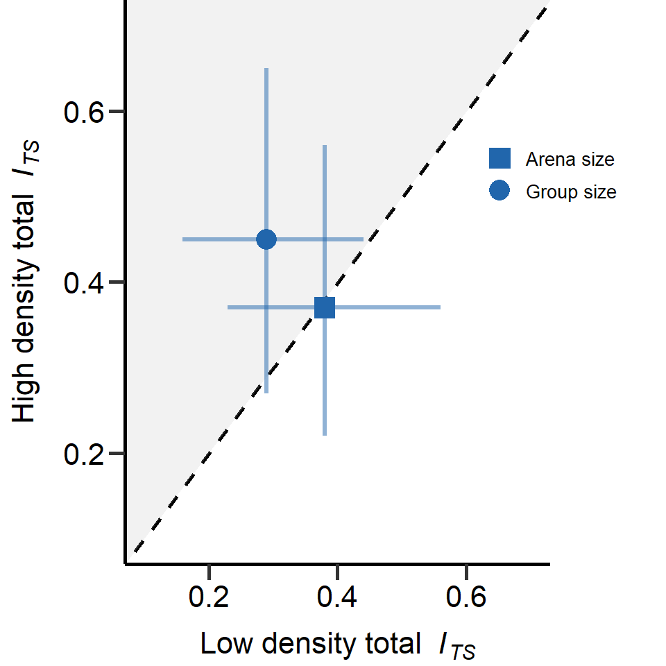

Figure S8: Total opportunity for sexual selection (ITS) in males for group and arena size treatment. Mean and 95%CI estimated via bootstrapping. Dashed lines mark equal effect size for both densities. In grey area metrics were larger under high density treatments. The x-/y-distance of means from dashed line is equal to the effect size of the treatment.

sessionInfo()

R version 4.2.0 (2022-04-22 ucrt)
Platform: x86_64-w64-mingw32/x64 (64-bit)
Running under: Windows 10 x64 (build 19045)

Matrix products: default

locale:
[1] LC_COLLATE=German_Germany.utf8  LC_CTYPE=German_Germany.utf8   
[3] LC_MONETARY=German_Germany.utf8 LC_NUMERIC=C                   
[5] LC_TIME=German_Germany.utf8    

attached base packages:
[1] grid      stats     graphics  grDevices utils     datasets  methods  
[8] base     

other attached packages:
 [1] knitr_1.42         ICC_2.4.0          data.table_1.14.8  boot_1.3-28       
 [5] RColorBrewer_1.1-3 car_3.1-1          carData_3.0-5      gridGraphics_0.5-1
 [9] cowplot_1.1.1      EnvStats_2.7.0     dplyr_1.1.0        readr_2.1.4       
[13] lmerTest_3.1-3     lme4_1.1-31        Matrix_1.5-3       gridExtra_2.3     
[17] ggplot2_3.4.1      ggeffects_1.2.0    workflowr_1.7.0   

loaded via a namespace (and not attached):
 [1] httr_1.4.5          sass_0.4.5          bit64_4.0.5        
 [4] vroom_1.6.1         jsonlite_1.8.4      splines_4.2.0      
 [7] bslib_0.4.2         getPass_0.2-2       highr_0.10         
[10] yaml_2.3.7          numDeriv_2016.8-1.1 pillar_1.8.1       
[13] lattice_0.20-45     glue_1.6.2          digest_0.6.31      
[16] promises_1.2.0.1    minqa_1.2.5         colorspace_2.1-0   
[19] htmltools_0.5.4     httpuv_1.6.9        pkgconfig_2.0.3    
[22] scales_1.2.1        processx_3.8.0      whisker_0.4.1      
[25] later_1.3.0         tzdb_0.3.0          git2r_0.31.0       
[28] tibble_3.2.0        generics_0.1.3      farver_2.1.1       
[31] ellipsis_0.3.2      cachem_1.0.7        withr_2.5.0        
[34] cli_3.6.1           magrittr_2.0.3      crayon_1.5.2       
[37] evaluate_0.20       ps_1.7.2            fs_1.6.1           
[40] fansi_1.0.4         nlme_3.1-157        MASS_7.3-56        
[43] tools_4.2.0         hms_1.1.2           lifecycle_1.0.3    
[46] stringr_1.5.0       munsell_0.5.0       callr_3.7.3        
[49] compiler_4.2.0      jquerylib_0.1.4     rlang_1.0.6        
[52] nloptr_2.0.3        rstudioapi_0.14     labeling_0.4.2     
[55] rmarkdown_2.20      gtable_0.3.1        abind_1.4-5        
[58] R6_2.5.1            fastmap_1.1.1       bit_4.0.5          
[61] utf8_1.2.3          rprojroot_2.0.3     stringi_1.7.12     
[64] parallel_4.2.0      Rcpp_1.0.10         vctrs_0.5.2        
[67] tidyselect_1.2.0    xfun_0.37

Population density affects sexual selection in an insect model